Abstract

The software industry necessitates early prediction of software defects for effective quality assessment and resource allocation. During the initial stages of the software development life cycle (SDLC), failure data is often unavailable. Consequently, the insights of domain experts can be crucial in estimating potential software defects during these early phases. This paper introduces a model designed to forecast software defects prior to the testing phase, emphasizing the structure of the software development process. The model is developed using metrics derived from early artifacts of the SDLC. The development and experimental aspects of the model are presented through the application of a Bayesian belief network (BBN). The qualitative aspects of software metrics, along with expert opinions, form the core of this methodology. To demonstrate the practicality and effectiveness of the proposed approach, ten datasets from real software projects have been utilized. The analysis and validation of predicted software defects, based on varying levels of uncertainty from domain experts, are compared against actual defect occurrences.

Introduction

I. INTRODUCTION

In the software industry, the predominant method for estimation is often referred to as "expert opinion" [1]. Numerous authors discussing software estimation highlight 'expert judgment' as a prevalent technique, which is frequently characterized as a form of 'guessing' [2]. Managers and decision-makers typically depend on expert insights when faced with uncertainty. This reliance may encompass facts or evidence recalled by the expert, deductions made regarding new or undocumented scenarios, and the synthesis of various information sources to tackle novel challenges [3]. Experts can facilitate decision-making by structuring problem frameworks, developing conceptual models, or choosing analytical methodologies. They may also provide estimates concerning variables or event outcomes, along with their associated uncertainties. Particularly in situations where time or resources are constrained, experts serve as a vital alternative source of information for decision-makers [4]. Expert opinion is grounded in specialized knowledge and extensive experience with relevant tasks. Cooke [5] observed that expert opinion has been utilized in numerous project developments over the years, manifesting in various forms such as value-based opinions, scenario-based opinions, and estimate-based opinions. Jorgensen [6] examined expert estimation in software development efforts and concluded that expert estimation remains the primary strategy for assessing the effort required in software development projects. In recent years, Bayesian Belief Networks (BBN) have gained popularity as a means of representing uncertain expert knowledge. Ouchi [7] asserted that the Bayesian method is arguably the most effective technique for integrating expert opinions. The literature [8-16] has proposed numerous prediction and estimation techniques within the software engineering domain utilizing BBN. The estimation of software defects during the development process has recently garnered significant interest from researchers [8-12].

The early identification of software defects during the initial stages of the software development life cycle (SDLC) is crucial for the software industry, as it promotes cost efficiency and effective resource management. Software metrics are integral to the process of defect estimation in these early phases of the SDLC. Research conducted by Zhang and Pham identified thirty-two factors that influence software reliability throughout all stages of development. Similarly, a study by Li et al. ranked various software reliability metrics based on their predictive capabilities, utilizing expert opinion to inform their assessments. Catal et al. conducted a systematic review of different software defect prediction models, emphasizing the role of software metrics. During the early phases of the SDLC, failure information is often derived from expert knowledge, which can be quantified through software metrics. It is important to note that many software metrics are inherently uncertain. The Bayesian belief network (BBN) is particularly effective in modeling such uncertainty, making it a valuable tool for predicting software defects in the early stages of the SDLC. The literature indicates that while expert estimations are valuable, they may require training for accurate communication. The Bayesian method stands out as a robust approach for integrating expert opinions.

Consequently, this paper employs a BBN approach to train expert opinions, yielding reliable estimations even when the expert knowledge is limited.

The subsequent sections of this paper are organized as follows. Section 2 provides an overview of the Bayesian belief network. The methodology proposed is detailed in Section 3. Section 4 presents case studies involving ten actual software projects. An analysis and validation of the proposed method are discussed in Section 5. Finally, Section 6 offers the conclusions drawn from this research.

II. BAYESIAN BELIEF NETWORK

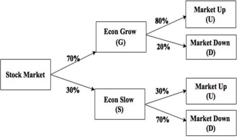
A Bayesian Belief Network (BBN) serves as a visual tool to illustrate the logical connections among various variables while also accounting for the uncertainty inherent in their interdependencies through the use of conditional probabilities. This framework is grounded in Bayes' theorem, which was formulated by the Reverend Thomas Bayes. An example illustrating Bayes' theorem is depicted in Figure 1, showcasing the logical relationships among five distinct variables.

In this context, the stock market is represented as having two descendants, G and S. Each of these descendants further leads to two additional descendants, U and D. Notably, the stock market itself does not possess any parent nodes, categorizing it as a root node. Conversely, U and D are identified as leaf nodes since they do not have any further descendants. The network diagram presented in Figure 1 is characterized as a directed acyclic graph, where the variables are denoted by nodes and the dependencies are illustrated through arcs. The fundamental mathematical expression of Bayes' theorem is articulated in Equation 1, which represents the basic formulation of Bayes' rule.

Figure 1. An example of BBN.

.Where P(G/U) is the posterior probability of hypothesis; P(U/G) is the likelihood of observed data: P(U) is the prior probability of hypothesis. Equation 2 is used for calculation the probability value when evidence is applied. For example if market is up, then what will be the the probability values of econ grow can be obtained using Equation (2).

III. PROPOSED METHODOLOGY

The following are the steps that our suggested methodology uses:
Step 1: Choose the most important software metrics from the SDLC's first stages.
Step 2: Build the BBN model with a few chosen software metrics. Step 3: Create an NPT (Node Probability Table) for each node. Step 4: Integrate the findings with the BBN model's compiled mode.
Step 5: Use the BBN model to determine the software defect's probabilistic value.
Step 6: Ask a domain expert to provide you with the optimistic and pessimistic software defect values.
Step 7: Calculate the anticipated cost of the software flaw.
While steps 1, 2, and 3 are taught in this part, case studies that are displayed in part will be used to demonstrate steps 4, 5, 6, and 7.

A. Selection of software Metrics

It is impractical to forecast software system reliability taking into account every metric that becomes available during the SDLC phases. But it's crucial to take into account the indicators that matter most in terms of reliability. Li et al. [19, 20] identified thirty software metrics that affect software reliability in relation to this problem. Through the process of eliciting expert opinions, these software measures were graded according to their predictive power. Based on research in [19, 20], our suggested BBN model includes seven of the most reliability-relevant software metrics that are taken from the early stages of the SDLC (i.e., requirements analysis, design, and coding phases). Table 1 displays the chosen best relevant measures for reliability.

B. Construct the BBN based on the selected metrics

The directed acyclic graph construction is the task of building the BBN. A large number of important SDLC phase-related components and their causal interactions need to be modeled in BBN.

Table 1. Selected software metrics

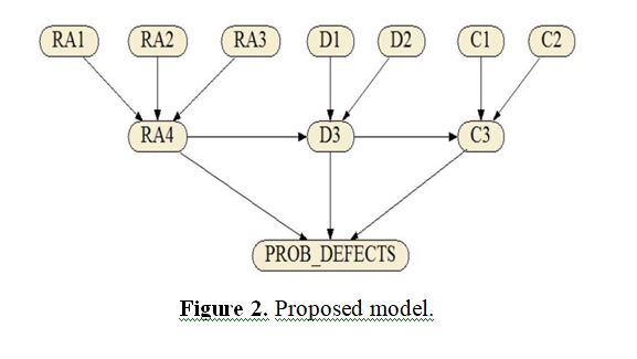
A methodical process for creating Bayesian causal maps was detailed by Nadkarni et al. [24]. The BBN model, depicted in Figure 2, is created using this process. To construct models, one tool that is employed is Netica [25]. The quality of SRS (RA4), quality of design (D3), and quality of code (C3) are determined using three metrics from the requirement analysis phase, two measurements from the design phase, and two metrics from the coding phase as input metrics. As a result, the model's output metrics are these three metrics: RA4, D3, and C3.

C. Construct the node probability table

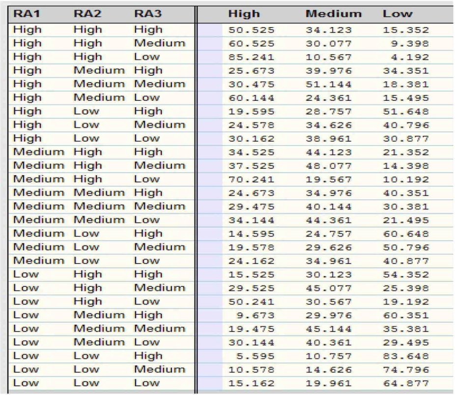
likelihood functions in BBN define the causal links between variables by taking as input a set of values from the parent nodes and computing the likelihood of the provided node. Tables, specifically node probability tables (NPTs), are frequently used to express these probability functions. One of the basic problems with the BBN is designing the NPT data. The literature has presented a number of approaches [26–30] for constructing NPT, although each approach is problem-specific. A method to create the NPT by domain experts and utilizing the qualitative value of software metrics was proposed by Kumar et al. [31]. This technique is based on fuzzy logic and the methodology of Tang et al. [30].

Figure 3. NPT of Quality of SRS.

IV. CASE STUDY

The suggested methodology is explained through ten case examples with illustrations. Table 2 replicates the data sets of 10 actual software projects, with H, M, and L denoting high, medium, and low, respectively, from [9].

Table 2. Qualitative value of software metrics

A. Apply the evidence to the compiled mode of BBN model

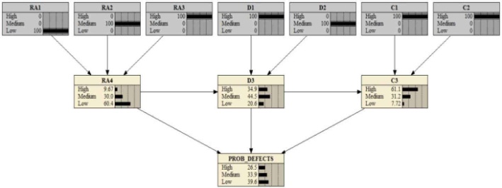
Applying the evidence to the compiled mode of the BBN model is required in order to determine the model's output. After creating the NPT for each node in the BBN model, the compile mode of the model may be acquired. The compiled mode of the BBN model is applied to the qualitative value of the software metrics (evidence) for case study 1 from Table 2. Figure 4 displays the final BBN model that was created after the evidence was applied.

Figure 4. Experimented result of case study 1.

B. Probabilistic value of software defect

To find the probabilistic value of a software error at the Low, Medium, and High levels, the evidence is applied to the compiled mode of the BBN Model. Applying the facts shown in Figure 4, the BBN model produces the software defect probability number for Case Study 1. In a similar manner, to ascertain the likelihood value of the software flaw, the data from the remaining nine cases are individually applied to the compliant mode of the BBN model. The probability values of software flaws in terms of High, Medium, and Low are shown in Table 3 and were produced by the BBN model.

Table 3. Probabilistic value of software defect

C. Obtain or Produce The Software Defect's Optimistic And Pessimistic Values From A Domain Expert.

A domain expert can provide you with the optimistic and pessimistic values of software defects based on his experience, education, knowledge of programming and technology, and the number of completed projects. The pessimistic (high) and optimistic (low) values of software defect are derived using the real software defect due to the unavailability of domain expert assessment. Based on real flaws, three distinct expert judgment uncertainty levels (20%, 40%, and 60%) are determined.
A high level deviates by 20%, 40%, and 60% from the actual defect, whereas a low level deviates by the same amounts from the actual defect. Table 4 displays the expert assessment of software flaw that was designed.

Table 4. Designed expert assessment of software defect

D. Estimate the predicted value of software defect

The probability value of a software defect derived from the BBN model, together with the pessimistic (high level) and optimistic (low level) values of software defects evaluated by a domain expert, are used to compute the anticipated value of the defect. Medium level is defined as the average of the high and low levels. The following formula is used to get the total number of anticipated software defects:

1) Case Study No: 1

Probability of software defect: High (0.265), Medium (0.339), Low (0.396).

 Expert assessment for software defect with 20% uncertainty level: Pessimistic (177.6), Optimistic (118.4).

Total number of predicted software defect

= (0.265 * 177.6) + (0.339 * 148) + (0.396 * 118.4) = 144.

Expert assessment for software defect with 40% uncertainty level: Pessimistic (207.2), Optimistic (88.8).

Total number of predicted software defect

= (0.265 * 207.2) + (0.339 * 148) + (0.396 * 88.8) = 140.

Expert assessment for software defect with 60% uncertainty level: Pessimistic (236.8), Optimistic (59.2).

Total number of predicted software defect

= (0.265 * 236.8) + (0.339 * 148) + (0.396 * 59.2) = 136.

Similarly, predicted value of software defect for rest 9 case studies is calculated. The complete result is shown in Table 5.

Table 5. Predicted value of software defect

V. MODEL VALIDATION AND RESULT ANALYSIS

Commonly used and recommended evaluation approaches for model validation have been implemented in order to validate the proposed model [9, 32]. Table 6 displays the comparing outcomes for various levels of uncertainty using Equations 3 through 7.

1) Root Mean Square Error (RMSE): RMSE is commonly used in measure of the differences between predicted values and actual values.

2) Normalized Root Mean Square Error (NRMSE): NRMSE is the ratio between the RMSE and the range of the actual values.

3) Mean Magnitude of Relative Error (MMRE): MMRE is the mean of absolute percentage errors and a measure of the spread of the variable z, where z = estimate/actual

4) Balanced mean magnitude of relative error (BMMRE): MMRE is unbalanced and penalizes overestimates more than underestimates. For this reason, a balanced mean magnitude of relative error measure is also considered which is as follows:

5) Co-efficient of determination (R)2: (R)2 gives a measure of how well actual outcomes replicated by the predicted outcome of proposed model.

Conclusion

This research uses a Bayesian belief network approach to evaluate the analysis of domain expert opinion in early software defect prediction. The creation of the BBN model makes use of the top seven reliability-relevant software metrics from the early stages of the software development life cycle model. To demonstrate the proposed model\'s applicability and usability, ten actual software project data sets have been applied to it. The real software defect and the anticipated defect using various domain expert uncertainty levels are compared. To verify the suggested methodology, RMSE, NRMSE, MMRE, BMMRE, and R2 has been employed. The precision of the forecast using varying degrees of uncertainty (20%, 40%, and 60%) is acceptable. Consequently the suggested method can be used to predict software defects in the early stages of software development, even in cases when the domain expert\'s degree of uncertainty exceeds 50%.

Copyright

Copyright © 2024 Prasanna Kumar, Dr. Kamdeo Prasad Yadav. This is an open access article distributed under the Creative Commons Attribution License, which permits unrestricted use, distribution, and reproduction in any medium, provided the original work is properly cited.