Artificial Neural Networks for Long-Bone Fracture Detection Based on X-Ray Image Contour Features

Abstract

Two contour-based fracture detection strategies are presented in the ensuing research. The programs are designed to help medical practitioners identify human long bone fractures from X-ray pictures. The line-based fracture detection systems suggested in [1] served as the foundation for the creation of the contour-based fracture. Convolutional Neural Networks (CNN) are widely used in current Computer Aided Diagnosis (CAD) systems to classify broken X-ray images. Even while the current CAD systems achieve excellent accuracy, doing so comes at a cost: a large volume of training data. By using identified contours in X-ray pictures, the suggested techniques aim to achieve high classification accuracy with little training data. Two methods exist for contour-based fracture detection. The first is the enhanced CHFB scheme, while the second is the Standard Contour Histogram Feature-Based (CHFB). The modified CHFB scheme differs from the other one in that it removes the detected flesh contours surrounding the leg region. The flesh shapes are identified as non-fractures automatically. To provide an accurate depiction of the image\'s edge objects, the contours are further adjusted. From every improved contour, a total of nineteen characteristics are retrieved. The frequency of specific identified gradients in the contour is the basis for eight of the nineteen characteristics. Additionally, the knee, leg, and foot regions are distinguished from one another using the contours\' 0~ gradient. The features serve as an input for the Artificial Neural Network (ANN) and are a condensed representation of the contour. Two assessments are used to evaluate the system. The first is an overall system performance foundation, which assesses the system using context-rich contours from the retrieved image. In the second evaluation, the system\'s ANN is solely assessed using randomly chosen contours; the context of the picture from which it was derived is absent. The evaluation is conducted using identical experimental setups for both the Standard CHFB and enhanced CHFB schemes. The enhanced CHFB scheme has an average accuracy of 82.98%, compared to the Standard CHFB scheme\'s 80.7% average system accuracy. Furthermore, utilizing recovered 0} gradients from broken contours, the hierarchical clustering approach is used to emphasize the fractured region within the X-ray picture.

Introduction

I. INTRODUCTION

Accurate detection is important in the medical arena for both medical practitioners and Computer Aided Diagnosis (CAD) systems. The author examines the development and state of CAD systems now in [2]. The CAD systems that identify the conditional qualities for certain medical problems are examined in this research. These include vertebral fractures, lung nodules, cardiomegaly, interstitial opacities, and interval alterations in chest radiographs. According to reports, CAD systems are classified as a "second opinion" before doctors make a final choice. The quantity of data needed to train artificial neural networks, which are used in standard CAD systems, determines the cost of an accurate image-based diagnostic. A fracture detection model is suggested by Kim, D.H. et al. [3] to look at how much learning can be conveyed in CNN networks. The main goal of the fracture detection was to identify wrist fractures from X-ray pictures. Five layers make CNN's construction: an input and output layer, two hidden layers, and a linked layer. 11,112 photos in total were used by the authors to train the model. Both fractured and non-fractured photos are included in the training. The model was tested using one hundred photos in total. There were fifty photos total—fifty with fractures and fifty without. According to the authors' findings, the sensitivity and specificity came out to be 0.9 and 0.88, respectively.

Furthermore, the model's AUC value of 0.954 shows that it has a good sensitivity for fracture diagnosis. A CAD system is presented by Brahim A. Et al. [4] for the early diagnosis of osteoarthritis (OA) in the knee. For the detection, the system makes use of machine learning techniques and knee X-ray imaging. The Fourier filter in the Fourier domain is used for pre-processing of the X-ray pictures. A dimensionality reduction approach called Independent Component Analysis (ICA) is used to choose among the retrieved features. The Naïve Bayes and random forest classifiers receive these chosen characteristics to classify and detect OA. The scientists used 1024 knee X-ray scans and obtained an accuracy of 84.98%.

For the categorization of specific circumstances, feature extraction is crucial. A deep feature fusion CAD system for lung nodule identification is proposed in [5]. A crucial component of CAD systems are features. The authors combine a range of characteristics from several CAD systems that use the traditional Convolutional Neural Networks (CNN). As dimensionality reduction is achieved by the application of Principal Component Analysis (PCA) to features, only important characteristics are considered. When compared to the traditional CNN, the scientists found that the deep feature fusion method produced better results for lung nodule detection.

Two Contour Histogram Feature-Based (CHFB) fracture detection schemes are suggested in this paper: an enhanced CHFB system and a standard CHFB method. The suggested line-based fracture detection systems in [1] serve as the foundation for the approaches. The enhanced CHFB technique differs from the other one in that it uses automatic contour recognition from surrounding skin. The strategy uses a feature-based methodology, whereby features are derived from the X-ray image's identified contours. therefore, lowering the quantity of data pictures needed for precise fracture diagnosis. From each contour, a total of nineteen characteristics are retrieved. In Section 2.7, the extracted characteristics are covered. PCA is used to analyze the features and identify the dominant contour feature or features. The feature(s) that distinguish a fractured contour from a non-fractured contour are indicated by the dominant feature(s), which is the feature(s) that contain the most information to offer insight. Section 2.9 goes into detail on how PCA is applied. The identified contours are adjusted to remove redundant data prior to feature extraction.

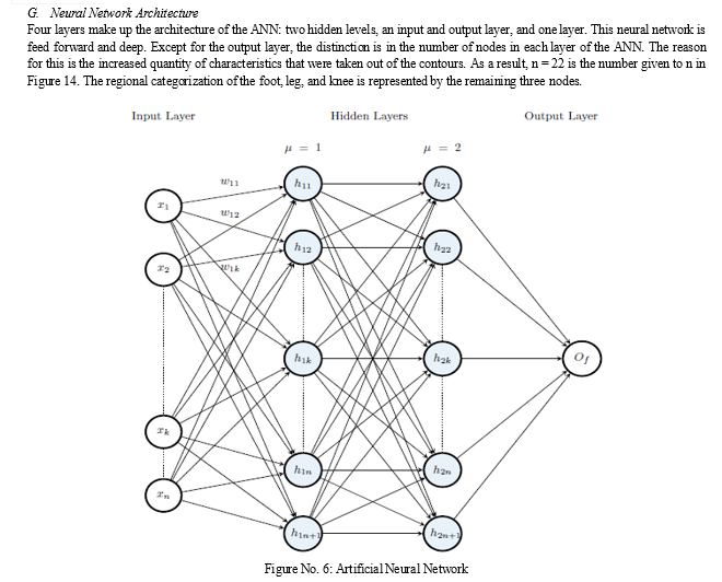
In Section 2.4, the contour refining process is covered in depth. Image segmentation is made possible by the contour's extra information. An X-ray picture has three unique sections: the knee, leg, and foot regions. The leg area is the focus once the three regions are divided by the picture segmentation procedure. In Section 2.5, the picture segmentation procedure is explained in depth. Four layers make up the ANN architecture for CHFB fracture detection: two hidden layers, an input and output layer, and one layer. Its ANN design is comparable to that of the ANN for the Standard and ADPO schemes. The number of nodes in each layer of the ANN, however, varies.

II. METHODOLOGY

A. An Overview of the Contour Histogram Feature-Based Fracture Detection System

The Standard and ADPO schemes' components are also present in the CHFB fracture detection scheme. The CHFB scheme differs from the others in that it includes an image segmentation component, further contouring refinement, and contour detection instead of line detection. To identify the dominating feature(s) that contribute to fractured and non-fractured contours, PCA is used to the extracted features. The architecture of the ANN and the training data that it uses to learn are the two parts that make up its training. When the ANN is executed, it detects broken contours and produces visual output results that allow for testing of the ANN's accuracy. Furthermore, a hierarchical clustering method using 0 gradient points taken from fragmented contours is used to identify the fractured region. Figure 1 shows a summary of the CHFB fracture detecting technique.

B. Image Enhancement

Prior to edge identification and contour extraction, the raw X-ray pictures are treated to guarantee improved and consistent image quality. Pixel equalization and the elimination of surrounding white space are steps in the picture enhancement process. unsharp masking, denoising, and gamma correction. The procedure makes sure that the long bone is the main focus of the X-ray picture and that every pixel is enhanced to provide a sharp contrast between the borders of the bones and every other pixel. The improved image is used to create a binary picture, which only has black and white pixels and highlights the boundaries of the bones. The Canny edge detection technique is used to detect edges. The OpenCV2.4 library provides the toolbox needed for Canny edge detection [6, 7].

C. Contour Extraction

The clever picture produced by the Canny edge detection method is used to identify the contours. The clever artwork features a dark background with highlighted borders. A series of points, (x; y), around picture edge objects is known as a contour [8]. As a result, the size of each detected contour changes according to the size of the image's edge object. The quantity of points that make up a contour determines its dimensions. Compared to the identified lines, the contour offers additional details about the items near the border of the image. This is since contours, which indicate picture edge objects discovered inside the X-ray image, are made up of more than two points. Nevertheless, redundancy is introduced by repeating points because the contour encircles the edge object. As a result, to remove the superfluous points that affect the depiction of the picture edge objects, the contours are further improved. The contours that were recovered from the X-ray picture are shown in Figure 2.

D. Contour Refinement Processing

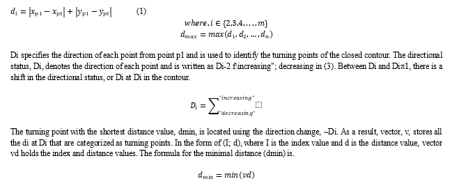
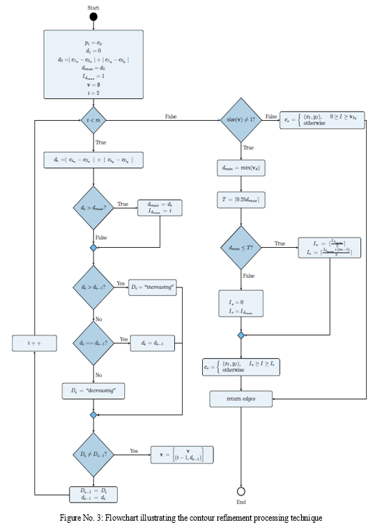
By removing repetitive locations, further contour processing aims to improve the contours. Because the contour encircling the picture edge objects is completed by repeated points, the contours are refined. As a result, removing the spots that are repeated lowers superfluous information and improves the representation of the image's edge object. Figure 3 shows a flow diagram of the contour refinement procedure. From the beginning index point, Is, the ending index value, Ie, specifies the point at which all the unique points inside the contour cease. Beyond Ie, every other point is a repeating point that makes up the entire closed contour. The greatest distance, dmax, between the contour's beginning point, p1, and all other points, pi, are computed to find Ie, where i 2 f2; 3; 4…. mg and m are the total number of points in the contour. (1) is used to compute the distance between each contour point and point p1, and (2) expresses the greatest distance.

E. Image Segmentation

The knee, leg, and foot regions are the three separate areas seen in X-rays of the lower human limb. The zones are divided from one another so that fracture identification from the X-ray picture may be done using contours (or lines). The goal of the separation approach is to separate the leg region's observed contours from all other areas. This is to prevent any mistake between the fragmented contours observed in the leg region and the contours detected in the knee and foot region. The separation process is predicated on the frequency analysis of gradients with 0~, 45~, 90~, and 135~ values. The identified contours are used to extract the gradients. The gradient between two neighboring contour points is calculated to get the gradients. The retrieved gradients are assessed by the frequency analysis at the corresponding vertical location in the X-ray picture.

Because of how the three sections are positioned, the interpretation is done using the image's vertical placements. In addition, the picture is divided into three independent parts by slicing it horizontally. The process is carried out by looking for patterns in the retrieved gradients. Further details on the location of the knee and foot regions within the picture are provided by the gradients. Consequently, compared to the contours within the leg area, the contours within the knee and foot region are more horizontally positioned.

F. Region Verification

The lower part of the limb (the foot) is at the bottom of the X-ray picture, which has a portrait orientation with the upper part of the lower limb (the knee area) at the top. As a result, the knee and foot area is verified using the y-values at 0} gradient. Since the other three gradients don't reveal anything about the regions, only the y-values at the 0} gradients are considered. The image's bottom right co-ordinate is (xmax; ymax), while the top left co-ordinate is (0; 0). The threshold values for the knee and foot areas are established using an adaptive method.

III. RESULT ANALYSIS

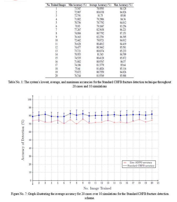
There are two assessments used to evaluate the Standard CHFB fracture detection method. While the second evaluation assesses the performance of the ANN, the first examines the scheme based on system performance. Contours with visual context are used in the initial assessment. Twenty pictures in all, along with the contours that go with them, are chosen at random to train the ANN. As a result, a total of 20 examples are available for the system's performance assessment. Since photos are chosen at random from a pool of 29 images for each example, there are 10 simulations total, which allows for a sufficient evaluation of the system. A picture typically has 112 contours, with a ratio of 1:3.70 between fractured and non-fractured contours. For every example, a total of 1,720 contours derived from 22 photos are analyzed. Out of the 1,720 contours, 1,433 are non-fractured and 287 are fractured. Table 2 presents the outcomes for every instance. Figure 6 presents the constancy of the detection accuracy visually. The system evaluation's accuracy falls between 74.3% to 85.17%. resulting in an accuracy of 80.7% on average.

The contours chosen by the second evaluation are at random and are not derived from any specific visual context. For each scenario, the ANN is trained using an equal number of fractured and non-fractured contours. As a result, 50% of the contours in the training data are fractured and 50% are not. The contours that are broken and those that are not broken are grouped in multiples of five for each of the 150 examples. As a result, 1,500 lines in total are employed to train the ANN. Figure 16 presents the findings. The findings indicate that the ANN's accuracy falls between 78% and 83%.

IV. DATA IMPROVEMENT

By using the x-value analysis on the contours' beginning and ending points to separate the surrounding flesh contours from the leg-bone contours, the Standard CHBF fractured detection technique is enhanced. Figure 18 gives an illustration of this. The outlines of the isolated flesh are automatically categorized as non-fractures. This reduces the ANN's training complexity. Furthermore, the skin contours are not included in the testing data set used to assess the ANN. If the skin contours are included in the testing data set, the ANN will not be fairly evaluated because it is not exposed to or knowledgeable about the flesh contours. Therefore, with the revised CHFB scheme, the average number of contours per picture is 108, and the fractured to non-fractured ratio is 1:3.99. Table 3 presents the results of the system evaluation of the revised CHFB scheme, which is based on 1,866 contours. 277 fractured and 1,433 non-fractured contours out of 1,866 total contours. The system's accuracy spans from 77.08% to 87.0%, resulting in an average accuracy of 82.98%. Figure 19 is a graphical representation of the accuracy. A little improvement in accuracy is seen for the modified CHFB scheme when comparing Figures 15 and 19. The accuracy increased to an average of 82.98% from an earlier 80.7% accuracy.

Figure 20 displays the AUC curve for the revised CHFB scheme, which has an AUC value of 0.8275. Compared to the Standard CHFB scheme, which has an AUC value of 0.8225, this is a little improvement. As a result, the enhanced CHFB system is more sensitive than the Standard CHFB scheme. Based on the observed data, the enhanced CHFB scheme achieves its maximum sensitivity at 0.21 FPR.

V. CRITICAL ANALYSIS

The enhanced CHFB scheme has an average accuracy of 84.03%, compared to 82.21% for the Standard CHFB scheme. Performance-wise, the enhanced CHFB scheme outperforms the standard CHFB scheme. Both methods' accuracy is determined using. The accuracy for both the system and ANN assessment does not account for the false positives and negatives that the system has discovered. The number of false positives and false negatives found indicates how sensitive the system's detection is. The enhanced CHFB system has the same proportion of false positives and false negatives, although having a higher detection accuracy than the Standard CHFB scheme. The standard CHFB scheme has a false positive to false negative ratio of 1:0.71, whereas the ratio for false positives to false negatives is 1:0.94.

Conclusion

Two contour-based fracture detection algorithms are shown in this chapter\'s conclusion. Using a Standard CHFB approach, all extracted contours are labeled and sent to an artificial neural network (ANN) with the purpose of classifying them as either fractured or non-fractured. The second is an enhanced CHFB scheme in which the leg-bone contours are obtained by performing additional processing to remove flesh contours within the leg area. As a result, the ANN only pays attention to shapes that are thought to be a component of the legbone. The ability of both systems to distinguish between fractured and non-fractured outlines with precision is measured. The ANN is given information about each contour through the extraction of a total of 19 characteristics from the contours. There are two assessments of accuracy used. In the initial assessment, which is a system evaluation, the ANN is given contours together with picture context. In the second assessment, the ANN is evaluated using contours without any background information about the corresponding picture. According to both accuracy tests, the Standard CHFB scheme\'s accuracy ranges from 74.3% to 85.17%, while the enhanced CHFB scheme\'s accuracy ranges from 77.08% to 87.0%. The enhanced CHFB scheme has a ratio of 1:0.94, whereas the standard CHFB scheme has a ratio of 1:0.71, according to additional examination of the false positive to false negative ratios for both systems. Consequently, compared to the Standard CHFB scheme, the Improved CHFB system has more false negatives. In the medical industry, false negatives are not accepted; yet, false negatives should be avoided for a system that generalizes for different inputs. In comparison to the Standard CHFB scheme, the Improved CHFB scheme provides greater sensitivity detection, albeit having a larger false negative to false positive ratio. This is acquired by examining the ROC graphs, which show the system\'s genuine positive detection performance\'s sensitivity over specificity. The AUC value of the Standard CHFB scheme is 0.8225, but the AUC value of the Improved CHFB scheme is 0.8275. Since the contours do not provide a clear picture of the fragmented region, the broken contours that have been found are further analyzed. This is a result of the fractured contours extending farther into the X-ray image\'s non-fractured areas. Using a hierarchical clustering technique, the broken zones are brought to light. To do this, the broken contours are identified, and their 0-degree gradients are extracted. The enhanced CHFB scheme\'s maximum accuracy is 89.07%; although, by enhancing the data labeling strategy, greater accuracy can be attained. An extra technique for deselecting non-fractured contours inside the chosen fractured area is part of the upgrade. For further advancements, new adaptive enhancements to the hierarchical clustering level selection are taken into consideration.

References

[1] Y. Yang and L. Cheng, “Long-Bone Fracture Detection using Artificial Neural Networks based online Features of X-ray Images,” arXiv:1902.07458 [cs], Feb. 2019, arXiv: 1902.07458. [Online]. Available: http://arxiv.org/abs/1902.07458 [Accessed: 2019-02-21] [2] K. Doi, “Computer-aided diagnosis in medical imaging: Historical review, current status and future potential,” Computerized Medical Imaging and Graphics, vol. 31, no. 4, pp. 198 – 211, 2007. [Online]. Available: http://www.sciencedirect.com/science/article/pii/S0895611107000262 [3] D. Kim and T. MacKinnon, “Artificial intelligence in fracture detection: transfer learning from deep convolutional neural networks,” Clinical radiology, vol. 73, no. 5, pp. 439–445, 2018. [4] A. Brahim, R. Jennane, R. Riad, T. Janvier, L. Khedher, H. Toumi, and E. Lespessailles, “A decision support tool for early detection of knee OsteoArthritis using X-ray imaging and machine learning: Data from the OsteoArthritis Initiative,” Computerized Medical Imaging and Graphics, vol. 73, pp. 11 – 18, 2019. [Online]. Available: http://www.sciencedirect.com/science/article/pii/S0895611119300035 [5] OpenCV. (2018, April) Canny edge detector — opencv 2.4.13.6 documentation. [Online]. Available: [Accessed: 2018-04-08] [6] B. Green, “Canny edge detection tutorial,” Retrieved: March, vol. 6, p. 2005, 2002. [7] OpenCV. (2019, Jan) findcontours. [Online]. Available: https://docs.opencv.org/2.4/modules/imgproc/doc/structural_analysis_and_shape_descriptors.html?highlight=findcontours#findcontours [Accessed: 2019-01-05] [8] I. T. Jolliffe, J. Cadima, and J. Cadima, “Principal component analysis: a review and recent developments,” Philosophical Transactions of the Royal Society A, vol. 374, no. 2065, p. 20150202, 2016. [9] S. Wold, K. Esbensen, and P. Geladi, “Principal component analysis,” Chemometrics and Intelligent Laboratory Systems, vol. 2, no. 1, pp. 37 – 52, 1987, proceedings of the Multivariate Statistical Workshop for Geologists and Geochemists. [Online]. Available: http://www.sciencedirect.com/science/article/pii/0169743987800849 [10] E. R. DeLong, D. M. DeLong, and D. L. Clarke-Pearson, “Comparing the areas under two or more correlated receiver operating characteristic curves: a nonparametric approach.” Biometrics, vol. 44, no. 3, pp. 837–845, 1988. [11] J. Bien and R. Tibshirani, “Hierarchical clustering with prototypes via minimax linkage,” Journal of the American Statistical Association, vol. 106, no. 495, pp. 1075–1084, 2011. [12] S. C. Johnson, “Hierarchical clustering schemes,” Psychometrika, vol. 32, no. 3, pp. 241–254, Sep. 1967. [Online]. Available: https://doi.org/10.1007/BF02289588 [13] “Hierarchical clustering - ALGLIB, C++ and C# library.” [Online]. Available: http://www.alglib.net/dataanalysis/clustering.php#downloadsection [Accessed: 2019-01-23] [14] K. Hajian-Tilaki, “Receiver operating characteristic (roc) curve analysis for medical diagnostic test evaluation,” Caspian journal of internal medicine, vol. 4, no. 2, p. 627, 201 [15] E. R. DeLong, D. M. DeLong, and D. L. Clarke-Pearson, “Comparing the areas under two or more correlated receiver operating characteristic curves: a nonparametric approach.” Biometrics, vol. 44, no. 3, pp. 837–845, 1988.

Copyright

Copyright © 2024 Ganesh Aravind Harkude. This is an open access article distributed under the Creative Commons Attribution License, which permits unrestricted use, distribution, and reproduction in any medium, provided the original work is properly cited.