CFD Analysis on Air Conditioning Effect Using K-Omega Model

Abstract

In this paper CFD analysis reveals the significance of cooling coil temperature, Reynolds Number, and Number of Occupants in the Chamber in the domain of maintaining ambient temperature. CFD Analysis used the regulation of any arbitrary office chamber using the Air conditioning effect. Governing equations consist of the Continuity equation, Energy Equation, and Naiver-Stokes Equation to understand the heating and cooling effect using Ansys. Unsteady Analysis is performed by varying several parameters like Reynolds Number, Number and Orientation of Cooling Coils. The strength of the Reynolds Number and the arrangement of cooling coils have a significant impact on maintaining the Temperature. K-omega SST model is best suited for near the wall flow region, say free surface flow region. According to the evaluation index of human thermal comfort, adopting K-omega SST turbulence model was more accurate compare to other models.

Introduction

I. INTRODUCTION

HVAC systems are more used in different types of buildings such as industrial, commercial, residential, and institutional buildings. The main mission of the HVAC system is to satisfy the thermal comfort of occupants by adjusting and changing the outdoor air conditions to the desired conditions of occupied buildings. Depending on outdoor conditions, the outdoor air is drawn into the buildings and heated or cooled before it is distributed into the occupied spaces, then it is exhausted to the ambient air or reused in the system. HVAC systems control the overall climate in the building. They also make the proper adjustments whenever we experience changes in outdoor temperature. During the winter season, the HVAC systems (mainly the boilers or heaters) work to keep the indoor temperature at a comfortable level. In hotter times of the season, the HVAC systems regulate air temperature by providing the necessary cooling to keep the entire building comfortable. Having a comfortable office climate increases the level of productivity and increases morale amongst the workers and employees. No employee will enjoy working in an office where it is freezing, or in an office where you frequently have to ignore your perspiration just to focus on your computer screen. Having a proper HVAC system installed is guaranteed to make your employees happy, hence, giving us better work results in return.

HVAC systems not only regulate the temperature inside the building, but they also improve the quality of air. The quality of air pertains to humidity, and a typical HVAC system will reduce the amount of humidity in the air so employees can continue enjoying a cosy and pleasant atmosphere at work. Proper HVAC systems are a worthy investment for any business or building owner because it gives you energy savings. HVAC systems today are automated. Given that your entire HVAC system operates in an automated system, proper adjustments will be made right when they are needed. This makes your energy consumption more efficient as it gets rid of energy wasted on improper settings. Computational fluid dynamics (CFD) is a branch of fluid mechanics that uses numerical analysis and data structures to analyze and solve problems that involve fluid flows. Computers are used to perform the calculations required to simulate the free-stream flow of the fluid, and the interaction of the fluid (liquids and gases) with surfaces defined by boundary conditions. With high-speed supercomputers, better solutions can be achieved, and are often required to solve the largest and most complex problems.

1. • It’s Cost Effective.
   • It gives much more flexibility to engineers.
   • The final analysis can be much deeper than with experimental testing.
   • The precision can be absurd.
   • It is not only useful for aerodynamics, but for other parts of the car too.

II. LITERATURE REVIEW

In the review the authors had the conducted the experiment in the traditional classrooms, study groups, and e-learning classrooms in a school and they did several trials by using different types of ventilation such as mixing ventilation, displacement ventilation and stratum ventilation. Among those ventilation, they have chosen the stratum ventilation to survey the indoor thermal comfort of a room with underflow air distribution in cold weather. The author had analysis the floor air supply and they did both means under and top floor air supply among those under air supply was better than the top floor air supply to get the same indoor thermal condition. Based on the previous studies, they have done with two types of the air distribution system including the bottom-supply mode and side-supply mode system. The simulating software of ANSYS was used to solve the following steady state, turbulent and governing equations for the flow field inside the experimental model room. Correct simulation of airflow in a room depends on the selection of turbulence, proper specifications of boundary conditions and quality of mesh. In being consistent with the experimental test, heat sources in the model room included four occupants, four computers on the desks and Figs the red cubes and cylinders were heat sources, the blue rectangles and circles were inlets, the green rectangles were outlets and the grey cubes were desks. The cooling load for each heat source (Chenxiao Zhenga, b, Shijun Youa, b, Huan Zhanga, b, Wandong Zhenga, c, ?, Xuejing Zhenga, Tianzheng Yea, ZeqinLiu, 2017)

Research paper key objective is to evaluate the effectiveness with which CFD can capture flow details near substantial flow obstructions, since this capability helps determine the usefulness of CFD. The simulation and calculation of the indoor environment and the PPD evaluation index are affected by three typical air conditioning supply modes there are Upper Supply-Bottom return, upper supply- Top Return and Bottom Supply-Top Return Analysing the trajectory change process of the streamline of it can be found that in the direction of supply air changed when it encountered the wall. The backflow was formed after the supply air hit the ground in the advancing process. In the backflow process, most of the airflow the advancing is discharged from the low outlet. A small part of airflow rose due to the influence of a heated source and formed a whirlpool due to being absorbed by the supply-air jet nearby. Overall, the occupied zone was basically in the recirculation zone. The supply air and the indoor air were fully mixed, and the air velocity of occupied zone was lower. The indoor air distribution, temperature, and velocity of the three air-supply modes were compared and analysed by simulation and calculation. The air-supply modes of the air-conditioned room included the patterns of upper-supply bottom- return, upper-supply top-return, and bottom-supply top-return. Fig. 3 provides the streamline of the room airflow of the three air-supply modes, which was the streamline of air that entered the model room from an air inlet in the steady state The PPD value reached the minimum neared the floor surface under the supply-air pattern of upper-supply top-return in the air-conditioned room, and the maximum value was obtained in the pattern of bottom supply top-return. The PPD value of the personal breathing zone (0.8–1.6 m) reached the minimum for the pattern of upper-supply top-return and obtained the maximum for the pattern of bottom-supply top-return. According to the evaluation index of human thermal comfort, adopting the pattern of upper-supply bottom-return was more comfortable. (Zeqin Liu,Ge Li &Chenxiao Zheng, 2014).

III. GOVERNING EQUATIONS AND METHODOLOGY

A. Continuity Equation

In equation 3.1 is continuity equation in computational fluid dynamics (CFD) is a fundamental principle that governs the conservation of mass in a fluid flow. It states that the mass flowing into a region of space must equal the mass flowing out of that region, with any change in mass due to sources or sinks within that region. The continuity equation can be written in mathematical form as follows  t = Time, ρ = Fluid density,  U = flow velocity vector field.

B. Navier Stokes Equation

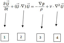
Term 1 signifies whether the flow is Steady or Unsteady ie., it tells us whether there is any disturbance in the flow or not, it is zero when there are no disturbances, and it has certain magnitude when there exist disturbances. Term 2 is a local acceleration term of the fluid particle in the field, it determines the velocity rate at which the fluid particle is travelling. It is a advection term. • Term 3 and 4 together constitute Diffusive terms. Term 3 is pressure term, this term signifies the difference between pressures at inlet and outlet and this is the one which drives the flow of fluid in flow field. Term 4 is viscous term which corresponds to the resistance to the flow it can be regarded as eddy viscosity. In Equation 3.2 states that the rate of change of momentum of a fluid element is equal to the sum of the forces acting on it. These forces include pressure, viscous forces, and body forces. The equation is nonlinear and often difficult to solve analytically, but can be solved numerically using computational fluid dynamics (CFD)

C. Energy Equation

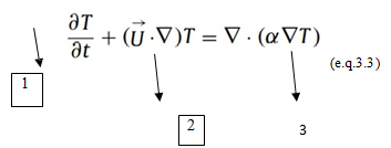
Term 1 is the variation of temperature with respect to Time. Term 2 is Advection term similar to Navier Stokes Equation. Term 3 is Conduction term. 

D. Methodology

1) Geometry

• Open the Fluent Ansys software and create geometry in a design modeler using the commands line, polyline, and circle.
• Give the dimensions to the geometry and convert the geometry into the surface by using the command surfaces from sketches.

• Give the named section to the geometry inlet, pipe, coil, occupants, table, and outlet.

2) Mesh

• Opening the mesh in the details of the mesh gives a smoothing factor as high and target skewness as 0.9.
• Give the growth rate as 0.9.
• Further geometry gives the edge-sized mesh.     
• Generate the mesh of the geometry by clicking on the generate mesh option.

Table 4.1: Details of mesh divisions

3) Setup

• Set the units of temperature to Celsius.
• Analysis type is pressure based and the time is transient.
• In the models on the energy and select the turbulent models as k-omega SST.
• In the materials select the fluid as air and the solid as copper.
• Initialize the solution.
• Initialize the solution by using the standard initialization method.
• Run calculations give the number of steps as 900, step size 0.1, and iteration as 5.
• Generate the residuals by running the calculations.
• Generate the temp contour and velocity vectors and particle path lines and plot the occupant the temp graphs by selecting the contours, vectors, path lines, and plot option in the results of the setup.

Table 4.2: Boundary conditions

4) Basic Structure of Geometry

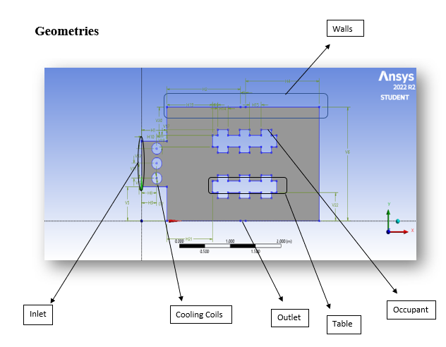
Figure 3.1. Model Geometry

Table 5.1 Dimensions

Figure-3.1 is a two-dimensional depiction of an actual three-dimensional office chamber.  It consists of one inlet, three cooling coils, 12 occupants, two outlets. The dimensions of the room is 3mx2m. Cooling Coils have a diameter of 0.2m. Based on the above geometry another three cases are modelled to perform further analysis.

5) Various Cases analyzed for the Analysis

Case1: Circular Shaped Coils (Linear orientation)                     Case2: Circular Shaped Coils (Staggered orientation)

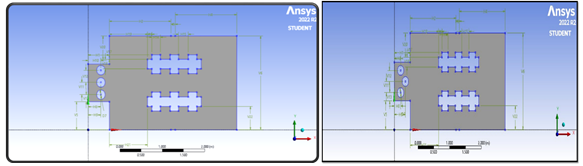
Fig. 3.2 Linear Orientation                                                 Fig. 3.3 Staggered Orientation

Case3: Elliptical Shaped Coils (Staggered orientation)           Case4: Elliptical Shaped Coils (Linear orientation)

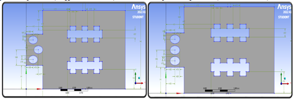
Fig. 3.4 Elliptical coils staggered Orientation         Fig. 3.5 Elliptical coils in linear position

6) Meshed geometries

Figure 3.6 Meshed Geometry 1                                 Figure 3.7 Meshed Geometry 2

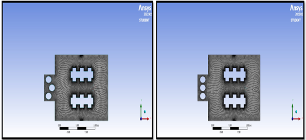
Fig. 3.8 Meshed Geometry 3                              Fig 3.9 Meshed Geometry 4

IV. RESULTS AND DISCUSSION

A. SST-K-Omega Model

1) Temperature Contours

In computational fluid dynamics (CFD) analysis, temperature contour plots are used to visualize the temperature distribution within a fluid or around a solid object. These contour plots provide a graphical representation of how temperature varies throughout the fluid or around the object under study.  The main use of temperature contour plots in CFD analysis is to identify regions of high and low temperatures within the fluid or around the solid object. This information is critical for engineers and scientists who are designing or optimizing systems that involve heat transfer, such as cooling systems for electronic components, combustion chambers, or heat exchangers.  By analyzing temperature contours, engineers can identify hot spots, cold spots, and areas where heat transfer is particularly efficient or inefficient. This information can then be used to refine the design of the system to improve performance, reduce energy consumption, or minimize thermal stress on materials. Overall, temperature contour plots are an important tool in CFD analysis because they allow engineers and scientists to visualize and understand complex temperature distributions in fluid systems, and to use this information to optimize the design of heat transfer systems.

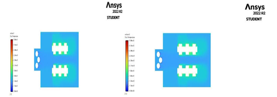
Fig. 4.1. Temperature contour Geometry 1                        Fig. 4.2 Temperature contour Geometry 2

In the fig 4.1 temperature contour the temperature at various regions can be easily visualized and the required cold spots and hot spots can be identified. For the above figure the highest temperature or hot spot is near the occupant which is nearly around 33.9 degrees centigrade, and the lowest temperature or cold spot is near the cooling coils which is nearly around 10.1 degrees centigrade. Similarly fig 4.2 explain the  temperature contour, the highest temperature or hot spot is near the occupant which is nearly around 34 degrees centigrade, and the lowest temperature or cold spot is near the cooling coils which is nearly around 9.48 degrees centigrade.

 
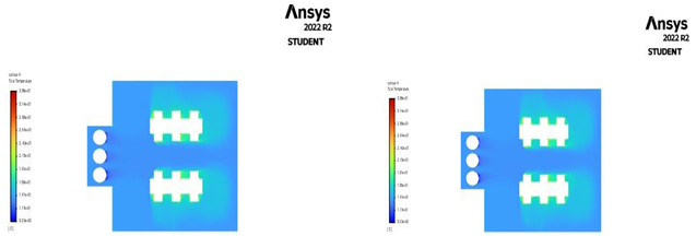
Fig. 4.3 Temperature contour Geometry 3             Fig.4.4 Temperature contour Geometry 4

Fig 4.3 shows that the temperature contour, the highest temperature or hot spot is near the occupant which is nearly around 33.7 degrees centigrade, and the lowest temperature or cold spot is near the cooling coils which is nearly around 8.33 degrees centigrade. Similarly in fig 4.4 temperature contour, the highest temperature or hot spot is near the occupant which is nearly around 33.8 degrees centigrade, and the lowest temperature or cold spot is near the cooling coils which is nearly around 9.4 degrees centigrade.

B. Path Lines in Chamber for Various Geometries

Particle path lines are a visualization tool used in computational fluid dynamics (CFD) analysis to track the movement of individual particles or fluid elements within a fluid flow. By tracing the paths of individual particles over time, engineers and scientists can gain a better understanding of the behavior and dynamics of fluid flows. The main use of particle path lines in CFD analysis is to identify flow patterns and areas of turbulence within a fluid flow. By examining the paths of individual particles, engineers can identify areas of high and low fluid velocities, as well as regions of recirculation and turbulence. Particle path lines can also be used to analyses the performance of fluid flow systems, such as pumps, turbines, or mixing vessels. By visualizing the movement of fluid particles, engineers can identify areas of inefficiency or areas where flow patterns may be causing unwanted effects, such as cavitation or erosion. In addition to their use in analyzing fluid flows, particle path lines can also be used to optimize the design of fluid flow systems. By analyzing the behavior of fluid particles under different conditions, engineers can adjust system geometry or operating parameters to improve performance or efficiency. Overall, particle path lines are an important tool in CFD analysis because they allow engineers and scientists to visualize and understand the complex behavior of fluid flows, and to use this information to optimize the design and performance of fluid flow systems.

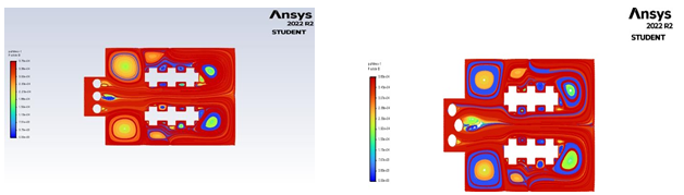
Fig 4.5 Path Lines Geometry 1                                        Fig. 4.6 Path Lines Geometry 2

 
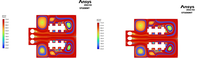
Figure 4.7 Path Lines Geometry 3                                        Figure 4.8 Path Lines Geometry 4

C. Velocity Contour for Various Geometries

Velocity contours are a visualization tool used in computational fluid dynamics (CFD) analysis to represent the distribution and magnitude of fluid velocities within a fluid flow. Velocity contours provide a graphical representation of how the velocity of the fluid varies throughout the fluid domain, allowing engineers and scientists to analyze and understand the behavior of fluid flows. The main use of velocity contours in CFD analysis is to identify areas of high and low fluid velocities within a fluid flow.

This information can then be used to refine the design of the system to improve performance or reduce the risk of damage. Velocity contours can also be used to analyze the effects of different operating conditions on fluid flow systems. By comparing velocity contours under different flow rates, temperatures, or pressure conditions, engineers can optimize the design of the system to achieve maximum efficiency or performance. Overall, velocity contours are an important tool in CFD analysis because they allow engineers and scientists to visualize and understand the complex behavior of fluid flows, and to use this information to optimize the design and performance of fluid flow systems.

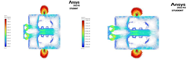
Fig. 4.9 Velocity Vector Geometry 1                       Fig. 4.10 Velocity Vector Geometry 2

In the figure 4.9, it has been identified the regions of low and high velocities, a major part of the room has a low magnitude of velocity nearly 2.17e-03 m/s and the region where there is high magnitude of velocity is near the outlet nearly 1.35e01 m/s and some regions of cooling coil, high magnitude of velocities may cause cavitation and must be taken care , also the regions with very low velocity must also be taken care in order to avoid turbulence.

Similarly in fig 6.2.10 shows that the identify the regions of low and high velocities from above figure , where high magnitude of velocity is near the outlet around 1.34e01 m/s and lowest magnitude of velocity around 2.55e-03 m/s.

 
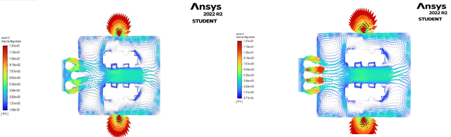
Fig.4.11 Velocity Vector Geometry 3                                        Fig.4.12 Velocity Vector Geometry 4

Figure 4.11shows that the regions of low and high velocities from above fig , the major part of the room has low magnitude of velocity and the region where there is  high magnitude of velocity is near the outlet i.e.., 12.2 m/s and the lowest magnitude of velocity is near the tables and the occupants i.e., around 8.30e-04 m/s. In figure 4.12 shows that the regions of low and high velocities from above fig, a major part of the room has low magnitude of velocity and the region where there is high magnitude of velocity is near the outlet i.e.., 12.1m/s and the lowest magnitude of velocity is near the tables and the occupants i.e., around 1.1e-03 m/s.

D. Occupant Static Temperature Graph

Static temperature graphs provide a graphical representation of how the temperature of the fluid varies throughout the fluid domain, allowing engineers and scientists to analyze and understand the behavior of fluid flows. The main purpose of static temperature graphs in CFD analysis is to identify areas of high and low temperature within a fluid flow. This information is important for engineers and scientists who are designing or optimizing systems that involve heat transfer, such as cooling systems for electronic components, combustion chambers, or heat exchangers.

By comparing static temperature graphs under different flow rates, temperatures, or pressure conditions, engineers can optimize the design of the system to achieve maximum efficiency or performance. Overall, static temperature graphs are an important tool in CFD analysis because they allow engineers and scientists to visualize and understand the complex behavior of temperature distributions in fluid systems, and to use this information to optimize the design and performance of heat transfer systems.

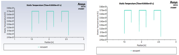
Fig.4.13 Static Temperature of occupant in Geometry 1   Fig.4.14 Static Temperature of Occupant in Geometry 2

The figure 4.13 is representing the temperature of three occupants at one end it can be seen that the occupant at a distance of 1.5m receives the cooling effect first and has an temperature of around 30.2 degree centigrade and the occupant at a distance of 2.3m i.e.., the third occupant has the least temperature among the three  occupants this is due the effect of wall near him, the occupant at that position receives the cooling effect directly as well as from the wall near him i.e.., the fluent reflects back after striking the wall and has temperature of around 29.3 degrees centigrade. In fig 4.14 it is same concept of wall effect applies to this case first occupant has temperature around 30.2 and third occupant has temperature around 29.3 degrees centigrade.

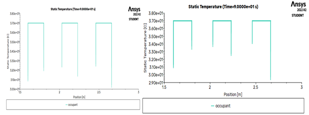
Fig.4.15 Static Temperature of occupant in Geometry 3   Fig.4.16 Static Temperature of occupant in Geometry 4

In figure 4.15 express the same concept of wall effect applies to this case first occupant has temperature around 30.2 and third occupant has temperature around 29.3 degrees centigrade. And in fig 4.16 shows the same concept of wall effect applies to this case, first occupant has temperature around 31.2 and third occupant has temperature around 29.3 degrees centigrade.

E. Total Occupant Temperature

Total temperature plot, also known as stagnation temperature plot, is a visualization tool used in computational fluid dynamics (CFD) analysis to represent the distribution and magnitude of the total temperature within a fluid flow. Total temperature is the sum of the static temperature and the kinetic energy of the fluid flow at a given point. The main use of total temperature plot in CFD analysis is to identify areas of high and low stagnation temperature within a fluid flow. This information is important for engineers and scientists who are designing or optimizing systems that involve high-speed fluid flows, such as gas turbines, jet engines, and rocket engines. By analyzing total temperature plots, engineers can identify areas of high stagnation temperature that may cause thermal stress on materials or lead to combustion, as well as areas of low stagnation temperature that may indicate regions of insufficient heat transfer. This information can then be used to refine the design of the system to improve performance or reduce the risk of damage. Total temperature plots can also be used to analyze the effects of different operating conditions on fluid flow systems. By comparing total temperature plots under different flow rates, temperatures, or pressure conditions, engineers can optimize the design of the system to achieve maximum efficiency or performance. Overall, total temperature plot is an important tool in CFD analysis because it allows engineers and scientists to visualize and understand the complex behavior of stagnation temperature distributions in fluid systems, and to use this information to optimize the design and performance of high-speed fluid flow systems.

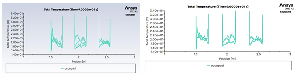
Fig. 4.17 Total Temperature of Occupant in Geometry 1 Fig 4.18 Total Temperature of Occupant in Geometry 2

Figure 4.17 shows the total temperature plot of three occupants at one end, the main purpose of the total temperature plot is to find the sum of static temperature and kinetic energy at a point. It is usually used for applications where there is high speed fluid flow. Here for the first occupant at 1.5 m the temperature is 26.2 degrees centigrade and for the third occupant it is 27.1 degrees centigrade. And the figure 4.18 represent the first occupant at 1.5 m the temperature is 32 degree centigrade and for the third occupant it is 31.8 degree centigrade.

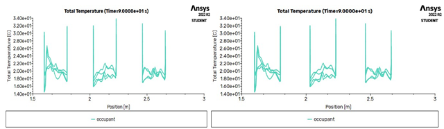
Fig.4.19 Total Temperature of Occupant in Geometry 3  Fig.4.20 Total Temperature of Occupant in Geometry 4

Figure 4.19 shows the first occupant at 1.5 m the temperature is 30.5 degree centigrade and for the third occupant it is 31.5 degree centigrade. Similarly the figure 4.20 shows the first occupant at 1.5 m the temperature is 32 degree centigrade and for the third occupant it is 31 degree centigrade.

F. Molecular Viscosity

In computational fluid dynamics (CFD) analysis, molecular viscosity plays an important role in determining the behavior of fluid flows. The main use of molecular viscosity in CFD analysis is to model the effects of fluid friction and the transfer of momentum within a fluid flow. The molecular viscosity of a fluid is used in the Navier-Stokes equations, which describe the motion of fluids, to determine the velocity and pressure distributions within a fluid flow. Molecular viscosity is particularly important in the simulation of turbulent flows, where the transfer of momentum between different regions of the flow can be very complex. By accurately modelling the molecular viscosity of the fluid, CFD simulations can provide a detailed understanding of the behavior of turbulent flows, which is important for designing and optimizing fluid flow systems such as aircraft wings, pumps, and turbines. In addition to its role in modelling fluid flow behavior, molecular viscosity is also used to determine the Reynolds number, a dimensionless parameter that characterizes the flow regime of a fluid. Overall, the use of molecular viscosity in CFD analysis is critical for accurately modelling the behavior of fluid flows and designing efficient and effective fluid flow systems.                

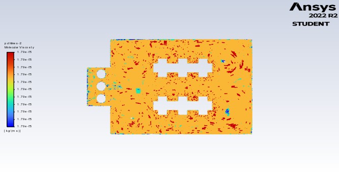
Fig.4.21 Molecular Viscosity in Geometry 1

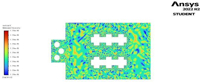
Fig. 4.22 Molecular Viscosity in Geometry 2

Figure 4.21 represents the molecular viscosity for the model, molecular viscosity is a, molecular viscosity is a parameter by which we can get information about fluid friction and momentum between particles, further it is also determining the Reynolds number which in turn is important parameter in determining the nature of the fluid flow. Majority y of the fluent is having a molecular viscosity around 1.75e-5 Pa-s. And in figure 4.22 same mentioned for the figure applies to this geometry as well, it has an molecular viscosity of 1.79e-5 Pa-s.

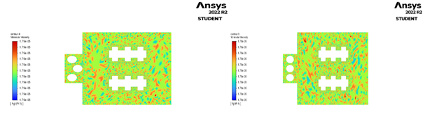
Fig.4.23 Molecular Viscosity in Geometry 3           Fig. 4.24 Molecular Viscosity in Geometry 4

Similarly, in fig 4.23 same mentioned for the figure applies to this geometry as well, it has an molecular viscosity of 1.79e-5 Pa-s. Similarly, in fig 6.1.24 same mentioned for the figure applies to this geometry as well, it has an molecular viscosity of 1.79e-5 Pa-s.

Conclusion

The Immersed Boundary Method (IBM) approach used in this paper provides a robust and efficient method for simulating complex geometries with moving boundaries, which can be useful in simulating fluid flow in a wide range of industrial and engineering applications. The paper presents a thorough validation of their numerical approach against previous experimental and numerical data (Takaki, R., Serizawa, A., & Fujisawa, N. (1997). Measurements of velocity and turbulence in the wake of a circular cylinder. Journal of Wind Engineering and Industrial Aerodynamics, 69-71, 189- 200.), demonstrating the accuracy and reliability of the IBM method in simulating the flow past a circular cylinder. Through the numerical Simulation of indoor thermal environment of the air-conditioned office chamber with load conditions and comparison of different cases by changing the shape of the cooling coils and orientation of the cooling coils in air-conditioning engineering, the following conclusions are given: 1) In the first geometry, from the temperature contour highest temperature in the office chamber after 90 seconds of air supply is 33.9oC. 2) In the Second geometry from the temperature contour highest temperature in the office chamber after 90 seconds of air supply is 33.8oC. 3) In the Third geometry, from the temperature contour highest temperature in the office chamber after 90 seconds of air supply is 33.7oC. 4) In the fourth geometry, from the temperature contour highest temperature in the office chamber after 90 seconds of air supply is 33.8oC. From temperatures of the different geometry cases, third geometry having the lowest temperature in the office chamber after 90 seconds of air supply. K-omega SST model is best suited for near the wall flow region, say free surface flow region. According to the evaluation index of human thermal comfort, adopting K-omega SST turbulence model was more accurate than K-epsilon turbulence model. In this analysis the same result is observed that SST K – omega is obtaining accurate results. 1) Reynolds number for circular shaped coils Re = ?VD/µ ? = density of air (kg/m3) V = flow velocity (m/s) D = Diameter of coil (m) µ = dynamic viscosity (kg/ms) Re = 1*2.5*0.14/1.79*10^-5 Re = 19553.07 2) Reynolds number for ellipse shaped coils Re = ?VD/µ Re = 1*2.5*0.18/1.79*10^-5 Re = 25139.66 3) Reynolds number is more per ellipse shaped coils. 4) If Reynolds\'s number is more the flow will be more turbulent. 5) Turbulence ensures proper mixing of fluid, as a result the higher is more cooling effect is obtained

References

[1] Chenxiao Zhenga, b, Shijun Youa,b , Huan Zhanga,b , Wandong Zhenga,c, Xuejing Zhenga, Tianzheng Yea , Zeqin Liud, Comparison of air-conditioning systems with bottom-supply and sidesupply modes in a typical office room, Journal of Applied Energy, Vo;.227, October 2018, Pp.304-311. [2] Zeqin Liu,Ge Li &Chenxiao Zheng, The simulation and calculation of indoor thermal environment and the PPD evaluation index affected by three typical air-conditioning supply modes, Journal of HVAC & R Research, Vol.20, Issue 3, April 2014. [3] J.D.Posner, C.R.Buchanan, D.Dunn-Rankin, Measurement and Prediction of Indoor Air Flow in a Model Room, Journal of Energy and Buildings Vol.35, Issue 5, June 2003, Pp.515-526. [4] Ranjit J. Singh, Abhilash J. Chandy, Numerical investigations of the development and suppression of the natural convection flow and heat transfer in the presence of electromagnetic force, International Journal of Heat and Mass Transfer Vol.157, August 2020, Pp.119-823. [5] Javad Taghinia, Md Mizanur Rahman, Timo Siikonen, Numerical simulation of airflow and temperature fields around an occupant in indoor environment, Journal of Energy and Buildings Vol.104, Issue 5, October 2015, Pp.199-207. [6] D Chatterjee, S K Gupta, B Mondal, Mixed convective transport in a lid-driven cavity containing a nano fluid and a rotating circular cylinder at the center. Int. Commun. Heat Mass Transfer 56 (2014) 71–78.

Copyright

Copyright © 2025 S. Deepak Reddy, P. Surendar Reddy, S Madhava Reddy. This is an open access article distributed under the Creative Commons Attribution License, which permits unrestricted use, distribution, and reproduction in any medium, provided the original work is properly cited.