“Climate Change Projections in Jammu and Kashmir under A1B, A2 & B2 Scenarios”

Abstract

The Global Climate Model (GCM) run at a coarse spatial resolution cannot be directly used for climate impact studies. Downscaling is required to extract the sub-grid and local scale information. The present study was undertaken to study the effect of climate change on weather parameters like maximum temperature, minimum temperature and precipitation for A1B, A2 and B2 scenarios. The study uses the Hadley centre coupled model (HadCM3) of the Intergovernmental Panel for Climate Change (IPCC) Forth Assessment Report. Thirty year weather data (1985-2015) obtained form Indian Metrological Department (IMD) Srinagar was used for the study. Statistical Downscaling Model (SDSM), R software and Artificial Neural Network (ANN) models were tested for the Srinagar area. This research investigates which among the three is better model for downscaling climate data for Srinagar area. The modelling results showed a first rate agreement between the experimental data and predicted values for temperature series with high coefficient of determination R2 values varying from (0.93-0.95) for different models. In case of precipitation R2 values varied from (0.08-0.249) for different models. The low values of coefficient of determination in precipitation time series are due to lot of uncertainty. occurrence of precipitation which could not be defined by the selected models. Based on Mean squared error (MSE), Root mean squared error (RMSE), Absolute average deviation (AAD), correlation coefficient and coefficient of determination, the R software performed better than the SDSM and ANN for maximum temperature, minimum temperature & precipitation. Thus R software was used for climate scenario generation. According to our simulated model, precipitation showed a decreasing trend whereas maximum and minimum temperatures showed an increasing trend. An overall increasing pattern of (9.81%) for A1B scenario, (15.24%) for A2 scenario & (10.32%) for B2 scenario for maximum temperature, (2.18%) for A1B scenario, (29.15%) for A2 scenario & (19.90%) for B2 scenario for minimum temperature and an overall decreasing pattern (22.60%) for A1B scenario, (17.23%) for A2 scenario & (7.11%) for B2 scenario for precipitation was noted.

Introduction

I. INTRODUCTION

Climate change is a change in the long-term weather patterns that characterize the regions of the world. Climate involves the average weather condition over a long period of time (Arthur Newell Strahler, 1960). Climate change in Intergovernmental Panel on Climate Change (IPCC) usage refers to any change in climate over time, whether due to natural variability or as a result of human activity. This usage refers from that of United Nations Framework Convention on Climate Change (UNFCCC) which defines climate change as, “a change of climate which is attributed directly or indirectly to human activity that alters the composition of the global atmosphere & which is in addition to natural climate variability observed over comparable time periods”. Climate change is not only a major global environmental problem, but also an issue of great concern to a developing country like India. Climate in a narrow sense is defined as “average weather”, or more rigorously, as the statistical description in terms of mean and variability of relevant quantities of weather parameters over a period of time ranging from months to thousands or millions of years. The classical period is 30 years, as defined by World Meteorological Organisation (WMO). The term “weather” refers to the short-term (daily) changes in temperature, wind, and/or precipitation of a region. Climate change is caused by factors that include oceanic processes (such as oceanic circulation), biotic processes, variations in solar radiation received by Earth, plate tectonics & volcanic eruptions, & human- induced alterations of the natural world; these latter effects are currently causing global warming, & “climate change” is often use According to the fifth Assessment Report (AR5) of the Intergovernmental panel on Climate Change (IPCC), global average temperature has shown a 0.85°C increase over the period of 1800-2012 (IPCC 2013), and a 0.18-0.74°C increase during the last 100 years (1906-2005) (IPCC 2007). This is probably due to the effects of industrialization that has increased greenhouse gas emissions.

However, the changes in extreme temperature events such as heat waves, severe winter and summer storms, hot and cold days, and hot and cold nights (Mastrandrea et al., 2011) can cause more severe impacts on human society and the natural environment.

The state of Jammu and Kashmir has also been presumed to suffer the consequences of global climate change. Jammu and Kashmir being one of the most sensitive ecological areas in Indian subcontinent has been at the vanguard of the discussions on climate change. It is clear that emissions of carbon dioxide and other gases and aerosols into the atmosphere from all sectors of human activities are central drivers of climate change. Their effects are now evident, and are becoming increasingly severe. A report prepared for the state’s department of ecology, environment and remote sensing in 2013 claimed average temperatures in the Kashmir valley has risen 1.45 degrees Celsius over two decades. As a result of rising temperatures in Kashmir, “over the past 50 years, hundreds of natural springs and streams have dried up, prompting people to encroach floodplains. 1.2. Emission Scenarios IPCC (2000) defines emission scenario as “images of the future or alternative futures”. They are neither forecasts nor predictions; rather all scenarios are one alternative image of how the future might reveal. A weather scenario must be representative, consistent and be a reasonable projection of possible future climates. It is not a forecast or prediction but it is an alternative image of how the future can be explained and its raw material is projected (IPCC, 2012). It should fulfil five criteria to be used for impact assessments and policy makers. According to IPCC (2012) report, these criteria are consistency with global projection, physical plausibility, applicability for impact assessments, representativeness and accessibility. Representative means that a scenario should be able to represent the

In this study the three scenarios A1B, A2 & B2 of HadCM3 model have been selected. Accordingly, the A1(low CO2 emission) scenario family describes a future world of very rapid economic growth, global population that peaks in mid-century and declines thereafter, and the rapid introduction of new and more efficient technologies. The A1 scenario family develops into three groups that describe alternative directions of technological change in the energy system (IPCC 2007). The three A1 groups are distinguished by their technological emphasis: fossil intensive (A1FI), non-fossil energy sources (A1T), or a balance across all sources (A1B) (where balanced is defined as not relying too heavily on one particular energy source, on the assumption that similar improvement rates apply to all energy supply and end-use technologies). Similarly, the A2 (medium high CO2 emission) scenario family describes a very heterogeneous world. The underlying theme is self-reliance and preservation of local identities. Fertility patterns across regions converge very slowly, which results in continuously increasing global population (IPCC 2007). The B2 (high CO2 emission) storyline and scenario family describes a world in which the emphasis is on local solutions to economic, social, and environmental sustainability. It is a world with continuously increasing global population at a rate lower than A2, intermediate levels of economic development. One of the most momentous potential concerns of weather prediction is hydrological components alteration and subsequent changes in lake/river water balance. Among the water balance components surface water inflow from ungauged and gauged catchments, precipitation and evaporation pattern alteration and their impact on water balance is not yet researched well. Therefore, this study investigates the pattern of climate change in the area

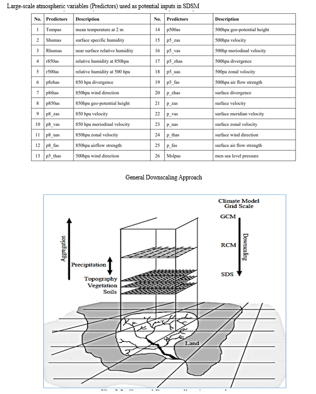
The present study is targeted to offer comprehensive simulations of extreme temperature events under three scenarios of HadCM3, A1B, A2 and B2, using Statistical Downscaling Model (SDSM), Artificial Neural Network (ANN) & R software in the area of Srinagar district with the following objectives: 1. To calibrate and validate the SDSM, ANN and R-software output for monthly parameters (i.e. precipitation, maximum temperature & minimum temperature) with observed patterns from meteorological station records. To analyse/compare each model to find out the best fit model amongst the three and to downscale the A1B, A2 and B2 scenarios from the HadCM3 using best fit model obtained above from the investigation. To evaluate the future change patterns of the best model for maximum, minimum temperature and precipitation

II. MATERIALS AND METHODS

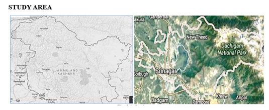
The present investigation entitled “Climate change projections in Srinagar under A1B, A2 and B2 scenarios” was undertaken in Srinagar, Jammu and Kashmir, during 2016- 2017. The details of the software used, techniques followed and materials used during the course of investigation are presented below. Study Area Description The study area for the survey was district Srinagar of Kashmir province, Jammu & Kashmir state (Fig). Srinagar is the summer capital of the Indian state of Jammu and Kashmir. It is situated in the centre of the Kashmir Valley on the banks of the Jhelum river and is surrounded by five districts. In the north it is flanked by Kargil and Ganderbal in the South by Pulwama, in the north-west by Budgam. The capital city of Srinagar is located 1585 metres above sea level. Srinagar has a humid subtropical climate, much cooler than what is found in much of the rest of India, due to its moderately high elevation and northerly position. The valley is surrounded by the Himalayas on all sides. Winters are cool, with daytime with daytime temperature averaging to 2.5 °C, and drops below freezing at night.

Moderate to heavy snowfall occurs in winter and the only road that connects Srinagar with the rest of India may get blocked for a few days due to avalanches. Summers are warm with a July daytime average of 24.1 °C. 3.2

III. DATA REQUIREMENT

A. Meteorological Data (daily):

1. Precipitation (daily).
2. Temperature (Min and Max)

The daily weather parameters collected from Indian Meteorological Department (IMD) Srinagar are shown along with their units of measurement in Table . The parameters chosen for study in this setup are maximum temperature, minimum temperature, & precipitation. There is no particular reason behind this choice of weather parameters. The choice is made just to predict the temperature variable. 30 years (1985-2015) data have been used in this research.

The input parameters used for study are given in Table

Climate Models General Circulation Models (GCMs), represent physical processes in the atmosphere, ocean, cryosphere and land surface. These are the most advanced tools currently available for simulating the response of the global climate system to increasing greenhouse gas concentrations. While simpler models have also been used to provide globally- or regionally-averaged estimates of the climate response, only GCMs, possibly in conjunction with nested regional models.

General Circulation Models (GCMs) are restricted in their usefulness for local impact studies by their coarse spatial resolution (typically of the order 50,000 km2) and inability to resolve important sub-grid scale features such as clouds and topography. As a consequence, two sets of techniques have emerged as a means of deriving local-scale surface weather from regional-scale atmospheric predictor variables. Firstly, statistical downscaling is analogous to the “model output statistics” (MOS) and “perfect prog” approaches used for short-range numerical weather prediction. Secondly, Regional Climate Models (RCMs) simulate sub-GCM grid scale climate features dynamically using time-varying atmospheric conditions supplied by a GCM bounding a specified domain.

IV. MODELS USED 

Statistical Downscaling Model (SDSM) SDSM was developed by Dr. Robert L. Wilby and Dr. Christian W. Dawson in UK for assessing local climate change impacts using a robust statistical downscaling technique. It is a Windows-based decision support tool for the rapid development of single-site, ensemble scenarios of daily weather variables under present and future regional climate forcing (Wilby et al., 2002).

It performs the tasks required to statistically downscale climate model output, namely: quality control of input data; screening of candidate predictor variables; model calibration; synthesis of present weather data; generation of future climate scenarios; basic statistical and time series analyses; and graphing results (Fig.)

It can be used for all locations in the world. Its key outputs are the site specific daily scenarios for maximum and minimum temperatures, precipitation, and humidity. It also produces a range of statistical parameters such as variances, frequencies of extremes, spell lengths. Its key inputs are the quality observed daily data for the statistical models. Daily GCM outputs for large-scale variables for future climate to drive the models. The SDSM software reduces the task of statistically downscaling daily weather series into seven discrete steps:

 • Quality control and data transformation;

• Screening of predictor variables;

• Model calibration;

• Weather generation (using observed predictors);

• Statistical analyses;

• Graphing model output; and

• Scenario generation (using climate model predictors).

R (Programming Language)

R is an open source programming language and software environment for statistical computing and graphics that is supported by the R Foundation for Statistical Computing. The R language is widely used among statisticians and data miners for developing statistical software and data analysis (Saiz-Álvarez, 2016). R is an integrated suite of software facilities for data manipulation, calculation and graphical display. Among other things it has,

• an effective data handling and storage facility,

• a suite of operators for calculations on arrays, in particular matrices,

• a large, coherent, integrated collection of intermediate tools for data analysis,

• graphical facilities for data analysis and display either directly at the computer or on hardcopy,

The source code for the R software environment is written primarily in C.

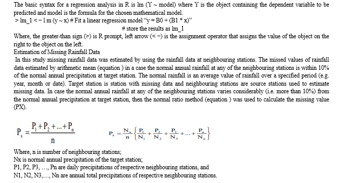
The basic installation (for Linux, Windows or Mac) contains a powerful set of tools for most purposes. For regression analysis, R uses lm ( ) command function.

V. SDSM CLIMATE SCENARIO GENERATION

The statistical test (i.e. t-test) was used to calculate a p-value, which is used to accept or reject the hypotheses that the two sets of data (i.e. observed and simulated) could have similar or the same statistical properties. Significant differences between the simulated and observed climate data may arise from the errors in the observed data, model smoothing of the observed data or random error.

A. Artificial Neural Network Processing

Experimentally developed 25915 observations for each input and output variables were used for developing the models. The dataset was randomly divided into two disjoint subsets, namely, training set having 21900 observations (80%) and validation set (20%) consisting of 4015 observations.

In this study, back-propagation training function in the toolbox was used to train feed-forward neural network. There are generally four steps in the training process.

1. Data preprocessing i. Assemble the training data ii. Normalization
2. Training the Neural Network

a. Defining the input and output

b. Choosing the architecture of the neural network

c. Create the network object.

d. Training the network

3. Post training analysis.

4. . Future data synthesis.

  Data preprocessing

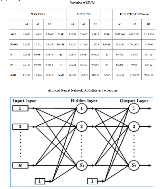
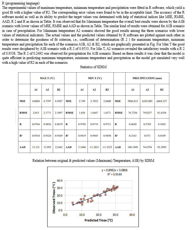
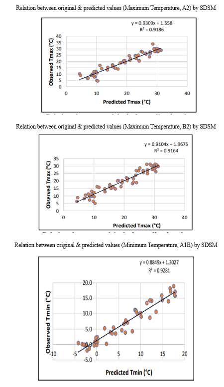
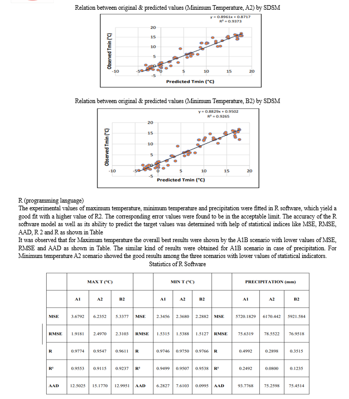
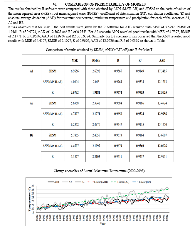
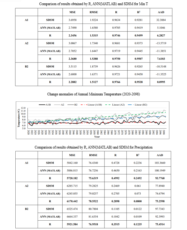
The above tables revealed that R-software model gave least values of MSE, RMSE and AAD and highest value of R2 among the three models. SDSM and ANN models also gave good results. The values obtained by SDSM and ANN are in agreement of the actual values, but the values of fitness obtained from R software model are closer to observed values as compared to values obtained from SDSM and ANN models. Thus, while SDSM and ANN models are good enough for prediction, R software model is most efficient in predicting the maximum temperature, minimum temperature and precipitation giving values closer to the observed values than the other two models.

Thus, the R software model is used for future weather prediction

VII. FUTURE PROJECTED CHANGES

The term anomaly means a deviation of future climate condition from a baseline period (1985-2015) climate condition. In this study baseline period climatic condition is analysed based on meteorological station records of the study area. Positive anomaly indicates an increase from the baseline period value, while a negative anomaly indicates decrease from the baseline period value. The anomaly of monthly precipitation is calculated as the difference from future monthly average precipitation to the baseline period (1985-2015) monthly average precipitation values (Figs.), The temperature is also calculated in the same way precipitation is calculated.

Conclusion

In this study SDSM, ANN & R modelling was carried out to study the climate change over the Srinagar area for a period of (2020-2098). SDSM, ANN & R models were developed & tested for their performance on the basis of results obtained from these models. The simulated values were compared with the original values to establish the precision of these models. The variation between the simulated and observed values of maximum, minimum and precipitation for A1B, A2 and B2 scenarios is represented by a set of graphs. The comparison between the models has been done on the basis of MSE, RMSE, AAD and R2 for their relative assessment The following conclusions were made: 1) The results obtained from SDSM, ANN & R showed good agreement between the observed data and simulated values with a high coefficient of determination. 2) The results obtained by the three models are however close to each other as well as to original values. • R modelling gave better results than SDSM and ANN models, revealing that the model was superior over other two models. 3) The modelling results showed a first-rate agreement between the experimental data and predicted values for temperature series with high coefficient of determination R 2 values varying from (0.93-0.95) for different models. In case of precipitation R2 values varied from (0.08- 0.249) for different models. The low values of coefficient of determination in precipitation time series are due to lot of uncertainty in occurrence of precipitation which could not be defined by the selected models. The R modelling result showed best agreement between the observed data and simulated values with a high coefficient of determination. 4) The results established that the developed models were able to analyse the given data with very good performance, fewer parameters, and shorter calculation time. On comparing the simulated results with the observed data of the previous years (1985-2015) it is ascertained that: 5) An overall increasing pattern (9.81%) for A1B scenario, (15.24%) for A2 scenario & (10.32%) for B2 scenario in the monthly maximum temperature is noted particularly in January (98.50%) for A1B scenario, January (71.8%) for A2 scenario & January (63.5%) for B2 scenario, while a consistently minimum change is noted in the month of May (0.3%). 6) An overall increasing pattern (2.18%) for A1B scenario, (29.15%) for A2 scenario & (19.90%) for B2 scenario in the monthly minimum temperature is noted particularly in Feb (182.50%) for A1B scenario, Feb (888.75%) for A2 scenario & Feb (973.75%) for B2 scenario, while a consistently minimum change is noted in the month of July (1.0%) for A1B scenario, Sep (13.43%) for A2 scenario & Sep (4.45%) for B2 scenario. 7) An overall decreasing pattern (22.60%) for A1B scenario, (17.23%) for A2 scenario & (7.11%) for B2 scenario in the monthly precipitation is noted particularly in Oct (57.80%) for A1B scenario, Oct (45.8%) for A2 scenario & Nov (63.9%) for B2 scenario, while a consistently minimum change is noted in the month of Jan (5.4%) for A1B scenario, Jan (2.9%) for A2 scenario & Jan (1.6%) for B2 scenario

References

[1] Abdellatif, M., Atherton, W. and Alkhaddar, R. 2013. A hybrid generalised linear and Levenberg–Marquardt artificial neural network approach for downscaling future rainfall in North Western England. Hydrology Research 44(6): 1084-1101. [2] Abdulkadir, A. S. Salami, A. W. and Kareem, A. G. 2012. Artificial neural network modelling of rainfall in Ilorin, Kwara State, Nigeria. Journal of Research Information in Civil Engineering 9(1): 108-120. [3] Abhishek, K., Kumar, A., Ranjan, R. and Kumar, S., 2012, July. A rainfall prediction model using artificial neural network. In Control and System Graduate Research Colloquium (ICSGRC), 2012 IEEE (pp. 82-87). IEEE. [4] Afifi, A. A. and Clark, V. 1996. Computer-Aided Multivariate Analysis, Third Edition, Chapman & Hall. Biometrical Journal 39(7): 875-876. [5] Aherne, J., Futter, M. N. and Dillon, P. J. 2007. The impacts of future climate change and sulphur emission reductions on acidification recovery at Plastic Lake, Ontario. Hydrology and Earth System Sciences Discussions 4(5): 3027-3054. [6] Ahmad, R. and Shabanlou, S. 2012. Climate Index Changes in Future by using SDSM in Kermanshah, Iran. Journal of Environmental Research and Development 7(1): 37-44. [7] Anandhi, A., Srinivas, V. V., Nanjundiah, R. S. and Kumar, D. N. 2008. Downscaling precipitation to river basin in India for IPCC SRES scenarios using support vector machine. International Journal of Climatology 28(3): 401-420. [8] Arti, R. N. and Pathan, S. K. 2012. Weather classification and forecasting using ii back propagation feed-forward neural network. International Journal of Scientific and Research Publications 2: 12. [9] Bas, D. and Boyaci, I.H. 2007. Modelling and optimization II: comparison of estimation capabilities of response surface methodology with artificial neural networks in a biochemical reaction. Journal of Food Engineering 78(3): 846-854. [10] Benestad, R. E., Hanssen-Bauer, I. and Chen, D. 2008. Empirical-statistical downscaling. World Scientific Publishing Company. [11] Bhotmange, M. and Shastri, P. 2011. Application of artificial neural networks to food and fermentation technology. In Artificial Neural Networks-Industrial and Control Engineering Applications. [12] Bocchiola, D. and Diolaiuti, G. 2010. Evidence of climate change within the Adamello Glacier of Italy. Theoretical and applied climatology 100: 351- 369. [13] Campozano, L., Tenelanda, D., Sanchez, E., Samaniego, E. and Feyen, J. 2016. Comparison of statistical downscaling methods for monthly total precipitation: case study for the paute river basin in Southern Ecuador. Advances in Meteorology. [14] Cavazos, T. 1997. Downscaling large?scale circulation to local winter rainfall in north?eastern Mexico. International Journal of Climatology 17(10): 1069- 1082. [15] Chaharborj, S. S., Borazjani, M. M. and Gheisari, Y. 2016. Predicting Climatic Meteorological Parameters by Using the Artificial Dynamics Neural Networks: Case Study, Bushehr City. Journal of Computer Science & Computational Mathematics 6(4): 113-119. [16] Chaleeraktrakoon, C. and Punlum, P. 2010. Statistical analysis and downscaling for the min, average and max daily-temperatures of the Chi and Mun River Basins. Thammasat. International Journal of Science and Technology 15: 64-81. [17] Cheema, S. B., Rasul, G., Ali, G. and Kazmi, D. H. 2011. A comparison of minimum temperature trends with model projections. Pakistan Journal of Meteorology 8(15): 39-52. [18] Christensen, J. H., Hewitson, B., Busuioc, A., Chen, A., Gao, X., Held, R., Jones, R., Kolli, R. K., Kwon, W. K., Laprise, R. and Magaña Rueda, V. 2007. Regional climate projections. In Climate Change, 2007: The Physical Science Basis. Contribution of Working group I to the Fourth Assessment Report of the Intergovernmental Panel on Climate Change, University Press, Cambridge, Chapter 11 (pp. 847-940). [19] Chu, J. T., Xia, J., Xu, C. Y. and Singh, V. P. 2010. Statistical downscaling of daily mean temperature, pan evaporation and precipitation for climate change scenarios in Haihe River, China. Theoretical and Applied Climatology 99: 149-161. [20] Combalicer, E. A., Cruz, R. V. O., Lee, S. and Im, S. 2010. Assessing climate change impacts on water balance in the Mount Makiling forest, Philippines. Journal of earth system science 119(3): 265-283. [21] Crowell, K. L. 2008. Precipitation prediction using artificial neural networks [22] Dibike, Y. B. and Coulibaly, P. 2005. Hydrologic impact of climate change in the Saguenay watershed: comparison of downscaling methods and hydrologic models. Journal of hydrology, 307: 145-163. [23] Dorji, S., Herath, S. and Mishra, B. K., 2017. Future Climate of Colombo iv Downscaled with SDSM-Neural Network. Climate 5(1): 24. [24] Duhan, D. and Pandey, A. 2015. Statistical downscaling of temperature using three techniques in the Tons River basin in Central India. Theoretical and applied climatology 121: 605-622. [25] Esfandiari, D. F., Hosseini, S. A., Azadi, M. M. and Hejazizadeh, Z. 2011. Prediction of Monthly Average Temperature Through Artificial Neural Network Multi-Layer Perceptron (MLP) Geography 8(27): 45-65. [26] Gagnon, S., Singh, B., Rousselle, J. and Roy, L. 2005. An application of the statistical downscaling model (SDSM) to simulate climatic data for streamflow modelling in Québec. Canadian Water Resources Journal, 30(4): 297-314. [27] Ghaffari, A., Abdollahi, H., Khoshayand, M. R., Soltani-Bozchalooi, I., Dadgar, A. and Rafiee-Tehrani, M. 2006. Performance comparison of neural network training algorithms in modelling of bimodal drug delivery. International Journal of Pharmaceutics 327(1-2): 126-138. [28] Golabi, M., Radmanesh, F., Akhondali, A. and Kashefipoor, M. 2013. Prediction of seasonal precipitation using artificial neural networks. Journal of Basic and Applied Scientific Research pp. 589-595. [29] Goyal, M. K., Burn, D. H. and Ojha, C. S. P. 2012. Statistical downscaling of temperatures under climate change scenarios for Thames river basin, Canada. International Journal of Global Warming 4(1):13-30. [30] Hashmi, M. Z., Shamseldin, A. Y. and Melville, B. W. 2011. Comparison of SDSM and LARS-WG for simulation and downscaling of extreme precipitation events in a watershed. Stochastic Environmental Research and Risk Assessment 25(4): 475-484

Copyright

Copyright © 2024 Dr. Bashir Ahmad Pandit. This is an open access article distributed under the Creative Commons Attribution License, which permits unrestricted use, distribution, and reproduction in any medium, provided the original work is properly cited.