Comparison Between Multi Epipolar Geometry and Conformal 2d Transformation-Based Filters for Optical Robot Navigation

Abstract

This research paper comes in a series of comparisons between the Multi Epipolar Geometry-based Filter (M-EGF) and the common filters that are extensively used in Optical Robot Navigation (ORN) for filtering the results of Automatic Image Matching (AIM). The accuracy of ORN depends mainly on the quality of the AIM results. Conformal 2D transformation-based Filter (C-2DF) is a common filter used in ORN applications. However, C-2DF is limited in terms of: time processing, disability to deal AIM data with significant number of outliers, dealing with images taking from different Depths Of Fields (DOF) and difficult view angles. M-EGF has been introduced recently by the author and compared with Single Epipolar Geometry based Filter (S-EGF), showing high ability to provide ORN with precise, trusted, outlier-free, and real time observations. In this paper, M-EGF has been compared with C-2DF using images captured by optical navigation system simulating ORN, which includes 3 cameras synchronized using GPS time. The performance of the two filters has been evaluated in different AIM environments and the automatically filtered results have been compared to precisely manually reviewed matched points using Matlap. Tests show that C-2DF has failed to deal with the AIM results in areas with open, narrow, and confused DOF. Also, they have failed to find out the right mathematical model in data with high rate of mismatched points and images with difficult view angles. C-2DF is also limited in its capability to deal with figures including different scales. With limited DOF and limited rate of errors, C-2DF has provided relatively sufficient results, which can be suitable for ORN in terms of quality and processing time. C-2DF overcomes S-EGF and M-EGF in terms of being not affected by errors in the Exterior Orientation Parameters (EOP) and Interior Orientation Elements (IOE) of cameras, as C-2DF depends on estimating the mathematical model parameters using only image points. Tests show that M-EGF is timesaving and be capable of dealing with any AIM findings, regardless DOF, vision angle and outliers level in used data. Also, unlike S-EGF, M-EGF is not affected in areas including lines parallel to the cameras base line. The results have proved that M-EGF is better than C-2DF, where it has provided error-free filtered matched points in all cases. This can be referred to the high control degree of this filter, where the percentage for the mismatched observation to pass through the three co-planarity conditions is theoretically nil. Tests show that errors in the cameras IOEs and EOPs affect the performance of M-EGF slightly in terms of rejection corrected matched points when they should be accepted, which can be mitigated considerably with professionally cameras calibration and EOP determination. Tests show that M-EGF is fast, restricted, reliable and error-free technique that suitable for real-time precise ORV-based applications.

Introduction

I. INTRODUCTION

ORN is a navigation technique used for determining changes in the location and orientation of robots relative to the surrounding environment. ORN is used in stationary and moving situations and based mainly on optical sensors [1]. ORN is based on obtaining dependable information about physical targets from captured images, and this discipline is simply defined as Photogrammetry. Analytical photogrammetry deals with   the mathematical functions, connected the main parameters used in ORN. These relationships can frequently take the forms of co-linearity equations or the co-planarity equations. [2]. The key parameters in photogrammetric equations are camera IOPs,  and EOPs, coordinates image points, Ground Control Points (GCP), and Object Space Coordinate (OSC) [3]. ORN technique is based on the main photogrammetric cases in both relative and absolute cases, including Space Resection (SR), Space Intersection (SI), Bundle Block Adjustment (BBA), and Self-Calibration Bundle Block Adjustment (SCBBA). ORN can be divided into two; the first includes the photogrammetric mathematical calculations, and the second includes extracting the identical points on images automatically using computer vision applications [3], [4].

In geomatic science, ORN is defined based on the type of sensors used in the processing, thus; with optical sensors, ORN is known as vision or image-based navigation, and using laser sensors, it known as laser scanning-based navigation. In computer sciences, ORN is known as Simultaneous Localization And Mapping (SLAM) [4]. Besides ORN, several navigation techniques are used based on the required task, type of application, surrounding environment, and outputs quality [3]. The other navigation methods can take the forms of satellite-based navigation, such as GPS [5], GPS/MEMS-based INS integration [6], GPS/delta positioning integration [7] and GPS delta positioning/MEMS-based INS integration [8], [9]. Integration between optical navigation with these navigation techniques is workable. ORN can be used in lots of applications, including security and safety, medical, and engineering. ORN is regarded as one of the mostly rapidly growing sectors, which is expected to occupy a serious place in the global markets [1].

The computer vision part of ORN depends mainly on finding out the matching points on the overlapping areas between images. Different techniques have been introduced by computer sciences for AIM, which are based on matching areas, features or relation. Cross-correlation and Least Squares Correlation (LSM) are the most familiar methods used in computer sciences for AIM. Recently, different robust feature detection techniques and algorithms have been developed, and used extensively in photogrammetry and computer vision applications [10], such as Scale Invariant Feature Transform (SIFT) [11], Principal Component Analysis (PCA)–SIFT [12], [13], and Speeded Up Robust Features (SURF) [14], [15].

Detecting outliers in AIM results by filtering mismatched image points is the key for accurate and reliable positioning and rotations in ORN, where the quality of the navigation solution is degraded depending on the level of outliers in the used observations. Identifying outliers is very important in ORN, as automation is used for measuring and determining the observations, and there is no opportunity for checking and investigating the data manually for gross errors. Outliers for multiple measurements of a single quantity can be detected easily using the normal distribution of the observational errors, which is not the case in ORN, where single measurements are fitted together during a least squares computations [1]. Different techniques are used for detecting gross errors in AIM data obtained by robust feature detection algorithms before used in ORN, which tend to be based on a well-defined mathematical function including the matched points across the two images. These mathematical functions can be classified into two main groups, namely: image points-independent models, and image points-dependent models. In the first, all parameters are known and fixed and AIM results are used in the model as inputs, accordingly, parameters estimation is not required. Independent models with no redundancy, such as co-linearity and co-planarity condition, can be used directly on the AIM results and certain threshold values are required for detecting outliers. S-EGF and M-EGF are clear examples on the first type of filtration models [1], [3], [4]. In image points-dependent models, such as 2D conformal and affine transformation methods, all parameters are unidentified and estimation steps are required firstly based on AIM results which are required to be filtered.  After estimating the model parameters, the model is applied on the rest of points for outliers detection. In the case of ORN, both types of filtration models can be used, where image points-independent models are based on recognized EOPs and IOEs of the cameras using co-planarity and co-linearity equations, and image points-dependent models are based on identified mathematical functions, such as 2D transformation methods, with unknown changeable parameters in each matching processing [3].

Random Sample Consensus (RANSAC) is regarded as one of the famous iterative technique used for estimating mathematical model parameters from a set of observations that includes outliers. It is a non-deterministic method that can provide results with a certain probability degree, depending essentially on the permissible number of iterations. RANSAC needs a set of observations, a well-defined mathematical model relating the observations, and confidence and flexibility ranges [1]. RANSAC consist of two iteratively repeated steps, where firstly, the minimum necessary number of observations, needed for determining the mathematical model parameters, is selected unsystematically from the whole data. The required parameters are determined using only the selected observations. As no redundancies are available, single solution can be obtained without any statistical indications for evaluating the used observations. In the second step, the mathematical model with the determined parameters in the first step is applied for the rest of observations. Based on that, observations can be differed into two sets, one for data fit the model within the acceptable identified threshold values, and the other group includes the rest of data not fitting the model and regarded as outliers. Step one is then reiterated using the outliers group, and the same process is carried out until no enough data for determining a new model remains in the outlier group. RUNSAC outputs is a number of groups, each one has its individual parameters for the same mathematical model. The parameters of the group that has the highest number of fit observations is regarded as the fit model, and its observations are inliers and others are outliers [1].

With a considerable number of iterations, RANSAC can provide consistent results, especially with reasonable number of outliers, and the possibility of finding the right model increase with more iterations, which makes the technique time consuming. On the other hand, using limited number of iterations can affect the quality of the obtained solution, and the fit solution may not be achieved of any kind.

The other limitation of RANSAC is the necessity of initial threshold values for detecting outliers, which should be precisely assessed, as they affect the performance in terms of making the model not flexible to the degree of rejection observations when they should be accepted and vice versa. This can be overcome by using maximum reasonable thresholds to guarantee including all fit observations as well as the adjacent outliers, and rejection all significant gross errors. Then, LSM is used with the selected observations to determine the best fit parameters and detecting outliers using simple techniques, such as Data Spoofing Method and based on LSM statistical testing indications.

This paper compares two AIM filtration techniques, which are M-EGF that introduced and discussed by the author in [1], [3] and C-2DF. M-EGF is an image points-independent mathematical model based on photogrammetric co-planarity conditions, whereas C-2DF is an image points-dependent mathematical model based on 2D conformal transformation equations. the same optical navigation based system used in [3], has been used for evaluating and testing the two filters in different AIM environments expected for ORN, including different DOF, view angles, type of routes, type of matching features, and rates of errors in observations. The performance of the two filters is evaluated based on the number of rejected points, that are correctly matched, and the number of accepted points, that are mismatched. The EOPs and IOEs of the cameras, as in [3], are determined precisely using using automatic coded targets and Australis Software.

II.   MATHEMATICAL DESCRIPTION

A. 2D Conformal Transformation-Based Filter (C-2DF)

2D transformation models can be used for detecting the mismatched points between images automatically, where the coordinate systems lie on plane surfaces. A conformal transformation is one of 2D transformation models, in which true shape is preserved after the transformation. A conformal transformation has the ability to work with changing in rotation, scale, and displacement. To apply 2D transformation model and find out the four main transformation parameters, namely: scale, rotation angle and two displacements, as a minimum, two points must be known in each coordinate system. 2D conformal transformation includes three stages, namely: determining the scale, then rotating, and finally two displacements. It is recommended for more precise results to use two points located away from each other which can help to absorb and contain the expected errors in the point coordinates. Using LSM with more points than the minimum number of points is also recommended for offering more consistent and robust results, and this is useful for detecting and removing outliers in observations based on LSM statistical testing information. In ORN, C-2DF can be used with RUNSAC technique for automatic detection of mismatched points, where the four parameters are estimated initially based on the minimum number of points (two points), and then applying the model on the other points, classifying them to inliers and outliers. The step is then reiterated with another two outlier pints and continues, resulting a number of groups, each one has its independent model parameters. The model that includes the more fitted observations is considered to be the main model and all other observations are regarded as outliers. RUNSAC with reasonable maximum threshold values is used at the beginning for giving the mathematical model more flexibility to accept the observations that are close to fit the model. After that, LSM can be used on these observations pass through the first step  to estimate the best fit parameters and removing the close undetected outliers based on statistical testing indicators. After removing these outliers, the remain observations can be bundled again for final parameters estimation. The mathematical model of C-2DF using RUNSAC and followed by LSM for any number of points (n) can be illustrated in the following steps and equations:

1. RUNSAC: Choosing two arbitrary points in image (1) and there matching points in image (2) as the lowest number of observations used for getting the four parameters of C-2DF. Equations (1.1 to 1.4) show the mathematical model of 2D conformal transformation:

E(A) = a * X(A) – b * Y(A) + T(E)                                                                                                           (1.1)

N(A) = a * Y(A) + b * X(A) + T(N)                                                                                                          (1.2)

E(B) = a * X(B) – b * Y(B) + T(E)                                                                                                           (1.3)

N(B) = a * Y(B) + b * X(B) + T(N)                                                                                                          (1.4)

Where,                                                      

a = S * cos(α)                                                                                                                                     (2.1)

b = S * sin(α)                                                                                                                                      (2.2)

S = (a2 + b2) 0.5                                                                                                                                   (2.3)

α = tan-1(b/a)                                                                                                                                     (2.4)

And,

T(E) , T(N)                       Displacement parameters of 2D conformal transformation

S                                   Scale changing

α                                   Rotation angle

X(A) , Y(A) , X(B) , Y(B)      The coordinates of points (A) & (B) in X-Y coordinate system

E(A) , N(A) , E(B) , N(B)     The coordinates of points (A) & (B) in E-N coordinate system

2. RUNSAC: Applying the model with the obtained parameters on the rest of points and categorizing the observations into two groups: inliers, that fit the model within the permissible limit values, and outliers, that do not do.

3. RUNSAC: Back to step (1), where another two points are chosen arbitrarily from the outliers group obtained in step (2). This procedure continues without stopping until facing one of the following cases: reaching the definite number of iterations, getting the model parameters with the maximum required number of fitted points, or the remaining outliers are less than 2 points. RUNSAC outputs are different groups, with independent 4 parameters for each one. The mathematical model that include the highest number of fitted points is considered to be the inlier model, and all others are outliers.

4. LSM: Because of threshold values that used for avoiding rejection points when they should be accepted, RUNSAC outputs are expected to include outliers. Therefore, points accepted by RANSAC are used again in LSM for determining the model parameters, and computing the residuals and the standard deviation of each observation from the covariance matrix of residuals. Equations (3.1 to 3.6) show example of C-2DF equations with redundancy and residuals are included to make them consistent:

E(A) + V E(A) = a * X(A) – b * Y(A) + T(E)                                                                                              (3.1)

N(A) + V N(A) = a * Y(A) + b * X(A) + T(N)                                                                                             (3.2)

E(B) + V E(B)  = a * X(B) – b * Y(B) + T(E)                                                                                             (3.3)

N(B) + V N(B) = a * Y(B) + b * X(B) + T(N)                                                                                             (3.4)

E(n) + V E(n)  = a * X(n) – b * Y(n) + T(E)                                                                                              (3.5)

N(n) + V N(n) = a * Y(n) + b * X(n) + T(N)                                                                                              (3.6)

Where,

T(E) , T(N) , S , α                            As in Equations. (1.1 to 1.4)           

X(A) , Y(A) , ……X(n) , Y(n)              The most probable computed values (error-free values)

E(A) , N(A) , ……E(n) , N(n)             Observed values including errors

In these equations, the residuals have been used just for E-N system coordinates, and X-Y system coordinates are regarded as error-free observations, which is not the case in AIM where mismatching is highly expected in the two images, especially in difficult matching environments.

Therefore, errors in all observations should be included and all observations are bundled together for accurate and stable geometry. Observation equation can be used to deal with the combined cases that including more than one observation in each equation.

This can be carried out by using one observation in each equation and using additional individual observation equation for each observation considered as error-free in the main equations. Additional equations to equations (3.1 to 3.6) should be used including the observations regarded as fixed values. Equations (4.1 to 4.6) show the additional equations includes the observed and the most probable values of each observation.

XO(A) + V(Xo(A)) =          X(A)                                                                                                                  (4.1)

YO(A) + V(Yo(A)) =          Y(A)                                                                                                                  (4.2)

XO(B) + V(Xo(B)) =          X(B)                                                                                                                  (4.3)

YO(B) + V(Yo(B)) =          Y(B)                                                                                                                  (4.4)

XO(n) + V(Xo(n)) =          X(n)                                                                                                                  (4.5)

YO(n) + V(Yo(n)) =           Y(n)                                                                                                                  (4.6)

Where,

XO(A) , YO(A) , ……, XO(n) , YO(n)                                 Error-free values

X (A) , Y (A) , ……, X (n) , Y (n)                                      Observed values including errors

V(Xo(A)) , V(Yo(A)) , ……,. V(Xo(n)) , V(Yo(n))                     Residual

These equations can be solved using LSM, providing wide range of useful statistical indicators. Equations (3.1 to 3.6) and (4.1 to 4.6) can be arranged in the matrixes of LSM as follows, and solved as shown:

A(n * m) * X(m *1) = L(n *1) + V(n *1)                                                                                                  (5)

X(m *1) = (AT(m * n) * W(n * n) * A(n * m))-1 * (AT(m * n) * W(n * n) * L(n *1))                                          (6)

Where,

n                                           The number of all observations (number of points * 4)

m                                          The number of unknowns (4 + number of points * 2)

A                                           Matrix of coefficients

AT                                         Matrix transpose

W                                          Matrix of observations weights

X                                           Matrix of unknowns

L                                           Matrix of constant terms

V                                           Matrix of residuals

A =      X(a)-Y(a)100000….00Y(a)X(a)010000….00X(b)-Y(b)100000….00Y(b)X(b)010000….00….….….….….….….….….00X(n)-Y(n)100000….00Y(n)X(n)010000….0000001000….0000000100….0000000010….0000000001….00….….….….….….….….….0000000000….1000000000….01                                       (7)

W =  unite matrix with diagonal of weight value of each observation:

[wX(A) ; wY(A) ; wX(B) ; wY(B) ; …….. ..….; wX(n) ; wY(n) ; wXO(A) ; wYO(A) ; wXO(B) ; wYO(B) ; ..….. .…..; wXO(n) ; wYO(n)]   (8)             

X = Vector matrix with one column of unknowns, including the 4 transformation parameters and the "true" values of X-Y system observations:

[a ; b ; T(N) ; T(E) ; X(A) ; Y(A) ; X(B) ; Y(B) ; …….…..; X(n) ; Y(n)]                                                                                                 (9)

L = Vector matrix with one column of:

[E(A) ; N(A) ; E(B) ; N(B) ; …… …..; E(n) ; N(n) ; XO(A) ; YO(A) ; XO(B) ; YO(B) ; …..; …..; XO(n) ; YO(n)]                                          (10)

V = Vector matrix with one column of observations:

[VE(A) ; VN(A) ; VE(B) ; VN(B) ; …….….., VE(n) ; VN(n) ; V(Xo(A)) ; V(Yo(A)) ; V(Xo(B)) ; V(Yo(B)) ; ….., ….., V(Xo(n)) ; V(Yo(n))]                 (11)

5. LSM: DSM and comparable outliers detection methods are suitable for using in this step, where the majority of gross errors have been removed in the RUNSAC steps. This step is suitable only for observations including low percentage of outliers. In DSM, the standard deviation of each observation residual is determined based on the observations covariance matrix obtained from LSM. The results of dividing the observation residual by its standard deviation should be less than (3), which depends on the required confidence level. With 99% confidence level, the critical value is nearly 2.6 and with 99.99%, it is almost 3. Observations locates outside the specified ranges are considered as outliers with (100% ­- confidence level) probability of rejection the observation when it should be accepted (type 1 error). After removing the remaining outliers from observations using LSM and DSM, all remaining observations are used again for determining final model parameters and these results are used directly in photogrammetric solutions for ORN, determining the position and orientation of the robot at the time of capturing the images. Equations (12, 13, 14) show the equations used in DSM to detect mismatched points form the LSM results.

CQV(n * n) = W-1(n * n) - A(n * m) *  (AT (m* n) * W (n * n)  * A (n * m)) * AT (m * n)                                                                                (12)

The slandered deviation (St V (1:n)) of residuals of observation from (1 to n) is the rote square of the diagonal of matrix CQV :

StV. (1:n) = [StV. E(A) ;  StV. N(A) ;  StV. E(B) ;  StV. N(B) ; …….…..;  StV. E(n) ;  StV. N(n) ;  StV. (Xo(A)) ;  StV. (Yo(A)) ;          StV. (Xo(B)) ;  StV. (Yo(B)) ; …….…..; StV. (Xo(n)) ;  StV. (Yo(n))]                                                                                                                                         (13)

w =  [VE(A)/StV. E(A) ;  VN(A)/StV. N(A) ;  VE(B)/StV. E(B) ;  VN(B)/StV. N(B) ; …….…..; VE(n)/StV. E(n) ; VN(n)/StV.N(n) ; V(Xo(A))/StV. (Xo(A)) ; V(Yo(A))/StV. (Yo(A)) ; V(Xo(B))/StV. (Xo(B)) ; V(Yo(B))/StV. (Yo(B)) ; …………; V(Xo(n))/StV.(Xo(n)) ; V(Yo(n))/StV. (Yo(n)) ]                               (14)

B. Multi-Epipolar Geometry-Based Filter (M-EGF)

M-EGF is an image points independent filter, introduced by the author in [3] for overcome the limitations of S-EGF and provide ORN with fast, robust and error-free inputs. The reader is referred to [1, 3, 4] for more information about M-EGF and all equations, explanations, and figures shown below are after Amami, 2022 [3]. In brief,  The idea of this filter is based on employing three cameras instead of two in robots, where three co-planarity conditions and three Epipolar geometries will be formed as shown in figure (1). The three co-planarity equations can be written as following [3]:

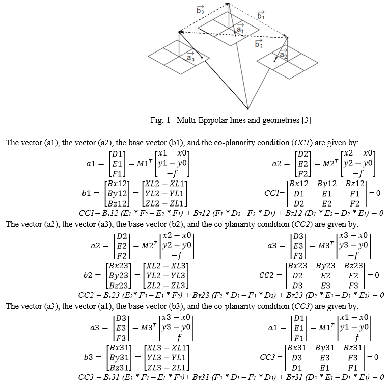
Where,                  M1, M2, M3          The rotation matrix of the third image to be corresponding to the reference coordinate system, and in case of relative orientation, rotations in the first matrix are used as zeros and relative values are used for the rotations of the second and third images.

x1, x2, x3                The "x" image coordinates of the same object on the three images.

y1, y2, y3                The "y" image coordinates of the same object on the three images.

XL1, YL1, ZL1             The coordinates of the first capturing station

XL2, YL2, ZL2          The coordinates of the second capturing station

XL3, YL3, ZL3          The coordinates of the third capturing station

f, x0, y0                  The camera IOEs (focal length and the coordinates of camera optical centre on the image).

M-EGF works according to the following procedure:

1. After matching each three images for each station using SURF algorithm, the results are uploaded to M-EGF.
2. The EOPs and IOEs of the three cameras are uploaded to M-EGF along with the their standard deviation values obtained from SCBBA in Australis software.
3. The co-planarity condition between each two images is applied, namely: CC1, CC2 & CC3
4. Passing the three point from the three co-planarity conditions proves beyond a reasonable doubt that it is inlier and correctly matched.
5. If the three matched points have failed to pass even one condition of the three conditions, the system will refuse the points and they are considered as mismatched points.

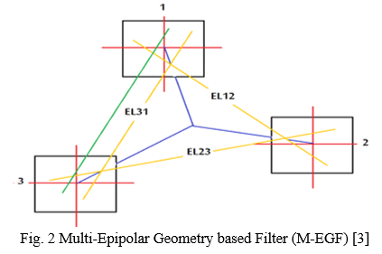
The high capability of M-EGF for removing the outliers from the matched points can be noted in figure (2). M-EGF consists of three S-EGF, the first is between image 1 & 2 (EL12), the second is between image 2 & 3 (EL23), and the last is between image 3 & 1 (EL31). EL12 is able to detect any mismatched points between images 1 &2, except those located on the extension of EL12 line. The same can be said for EL23 & EL31. If the mismatched points have passed the first filter (EL12 for example) as the point is located on the extension of EL12, the probability  of this point to pass through the other two filters is nearly zero. Theoretically, the only case for M-EGF to not detect the mismatched point between the three points can be explained as following:

a. Assume that there are three points (a1, a2, a3) in the three images (1, 2, 3), respectively. These points are obtained from SURF algorithm and required to be checked by M-EGF for being inliers or outliers.

b. a1 is outlier, located along the line EL12, and it distances away from the correct point by "d1".

c. a3 is outlier, located along the line EL23. and it distances away from the correct point by "d2"

d. The two distances "d1" and "d2" are equal, which makes the pseudo EL31 (the green line in figure 2) is exactly parallel to the original EL31 (the yellow line in figure 2).

So, it is clear from this assumption that the probability of passing any mismatching point from M-EGF is actually zero. Based on that, if precise values of the EOPs as well as IOEs for the three cameras are used with reasonable standard deviations, there is no chance mathematically to accept any points when it should be rejected and vice versa.

III. TESTING, RESULTS & DISCUSSION

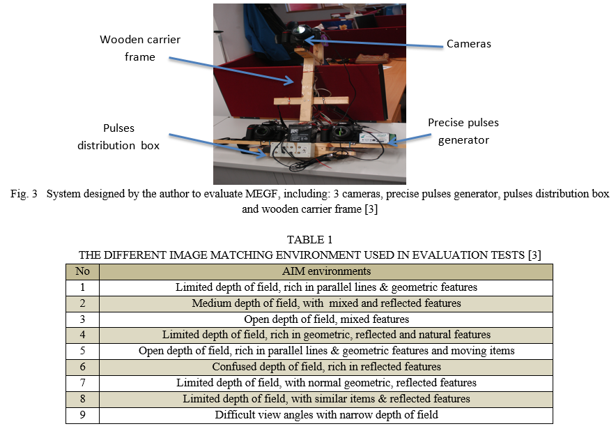
To evaluate the performance of the M-EGF comparing to C-2DF, the same system, tests and images, that used in [3] for comparing M-EGF and S-EGF, will be used in this paper. The system includes 3 cameras, connected to GPS based timing and pulsing devise via distribution box to synchronizing taking the three images. Figure (7) shows the system and main components. The IOEs as well as EOPs of the three cameras have been calibrated precisely using Australis Software via automated detection coded targets. Table (1) illustrates the different AIM environments used in evaluation tests. Figures (4), (5) and (6) show examples of different AIM environments and examples of passed mismatched points using C-2DF.

The evaluation technique used in this paper can be summarized in the following steps:

1. C-2DF has been developed in Matlab using RANSAC and LSM, where the inputs are the matched points and some statistical thresholds, whereas the results are two groups: inliers and outliers with the final 4 parameters of 2D conformal transformation. 
2. The results of M-EGF obtained in [3] have been used in this paper to be compared to C-2DF, as the same system, tests and images are in use.
3. The three images tacking in each environment have been automatically matched using adjusted SURF algorithm, taking the best 100 matched pints between each three images. 900 matched points between each three images have been used with 2700 overall total number of points  between the 27 pictures used in the tests.
4. These points have been manually and precisely checked and classified as inliers and outliers
5. The results of the two filters are automatically compared to the manually classified lists, giving the error percentage of the accepted points that should be rejected (E%-AC), and the rejected points that should be accepted (E%-RJ).
6. The processing time and the ability of the filter to deal with the inputs have been also taken into account for evaluating the three filters

Table (2) illustrates (E%-AC) and (E%-RJ) for M-EGF and C-2DF in the different AIM environments shown in table (1).

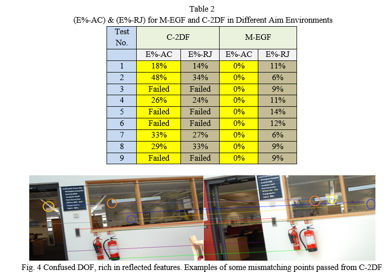
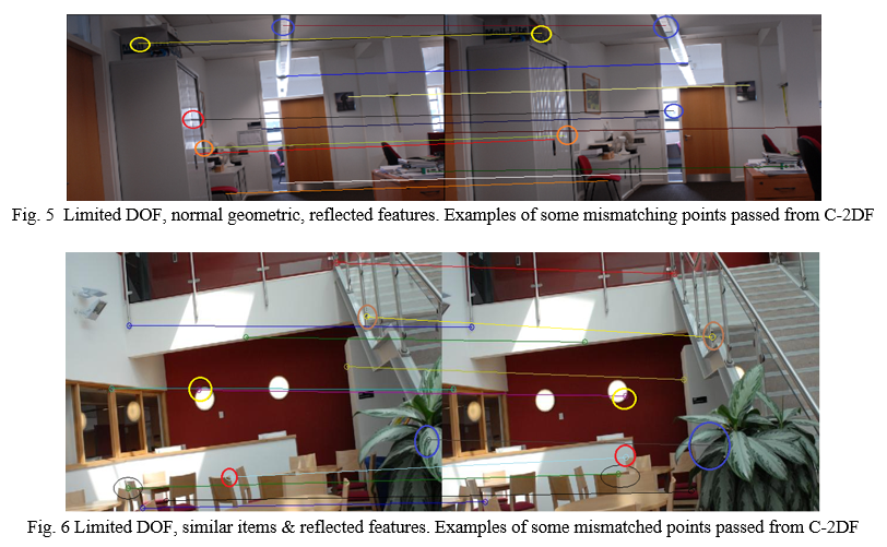
As clear from table (1) and table (2), in areas with open, narrow, and confused DOF, C-2DF has failed to filter the AIM results, which can be referred to the disability of RUNSAC and LSM to extract the right mathematical model based on these points. This can be attributed to the significant number of mismatching point used and/or changing the relationships between the points on the two images significantly with changing the depth distance between points in optical direction when dealing with different levels of DOF. On the other hand, M-EGF has shown high ability to deal with all inputs from all AIM environments, in spite of the outliers percentage in the used observations. This can be attributed to the main dependency of M-EGF on fixed mathematical models without the need for estimating any parameters as in the case of C-2DF. Also, DOF and similarity of matching features did not have any effects on the performance of M-EGF, where the filter is image point independent model. This means that factors that might affect the performance of AIM techniques tend to increase the number of outliers in the data required to be filtered, and this can just affect the image point dependent models, such as C-2DF. C-2DF has relatively shown good results in areas with limited DOF, where the relationships between points is nearly constant and changes in scale, rotations and displacements can be considered in the mathematical models. C-2DF has also difficulty to deal with images including difficult view angle and reflected features due to changing the scales, which can be seen in test (6). Furthermore, C-2DF is considerably affected by the complexity of AIM environment, where the filter depends principally on extracting the correct mathematical model that collects the biggest group of matched points obtained from AIM results. Increasing the number of mismatched points in the RANSAC inputs increases the difficulty of determining the correct geometric model, may perhaps give wrong one, or fails to get any relationship. The other limitation of C-2DF is the long processing time needed for estimating the right parameters of mathematical model, where both RUNSAC and LSM are iterative methods that need determining statistical testing for accurate results. This might reduce the chance of utilizing such filter for real time ORN applications.

As clear from the results, M-EGF has offered the best results in terms of  providing error-free filtered matching points in all tests, regardless the AIM environment and the number of errors in the inputted data. As the IOEs and EOPs of the cameras are not precise due to the manual fixing of the equipment on the wooden frame of the system, a number of corrected matched points have been rejected when they should be accepted, which can be avoided by precise and perfect manufacturing and calibrations.  Tests show that M-EGF is considerably timesaving comparing to C-2DF and as  a result suitable for real time ORN applications.  

IV. ACKNOWLEDGMENT

I would like to express my special thanks to my wife "Eng. Nagla Fadeil".

Conclusion

In this paper, two different filters, used for detecting outliers in AIM results, namely M-EGF and C-2DF have been tested and evaluated in various AIM environments with different level of outliers in observations. Results show that C-2DF has failed in areas with open, narrow, and confused DOF due to changing the relationships between the points extensively with rising the spaces in optical direction. Also, C-2DF has failed to determine the exact mathematical model with high percentage of outliers in images taken with difficult view angles. With limited DOF and limited outliers, C-2DF has shown E%-AC and E%-RJ higher than M-EGF, which reflects the limitation of utilizing this filter in precise ORN applications. The processing time is another limitation of C-2DF, where both RUNSAC and LSM used in this filter are iterative methods that need determining statistical indicators repetitively for accurate results. This procedure makes finding the right geometric model between hundreds of matched points is indeed time-consuming and unsuitable for real time ORN applications. M-EGF has proven its high power to deal with all inputs from all AIM environments, in spite of the outliers ratio in the used data. Also, M-EGF has shown high ability to overcome the effects of DOF, difficult view angles and similarity of matching features. Tests show that the quality of the cameras IOEs and EOPs can affect the performance of M-EGF in terms of rejection a number of corrected, and not otherwise, which can be avoided by precise and perfect manufacturing and calibrations. Tests show also that the dependency of M-EGF on fixed and known mathematical model help to make it considerably fast and time-effective comparing to C-2DF and, as a result, M-EGF is suitable for real-time ORN applications.

References

[1] M. M. Amami, “Low-Cost Vision-Based Personal Mobile Mapping System,” PhD thesis, University of Nottingham, UK. 2015. [2] J. C. McGlone, E. M. Mikhail, J. Bethel and M. Roy. Manual of photogrammetry. 5th ed., Bethesda, Md.: American Society of Photogrammetry and Remote Sensing. 2004. [3] M. M. Amami, “Comparison Between Multi & Single Epipolar Geometry-Based Filters for Optical Robot Navigation,” International Research Journal of Modernization in Engineering Technology and Science, vol. 4, issue 3, March. 2022. [4] M. M. Amami, M. J. Smith, and N. Kokkas, “Low Cost Vision Based Personal Mobile Mapping System,” ISPRS- International Archives of The Photogrammetry, Remote Sensing and Spatial Information Sciences, XL-3/W1, pp. 1-6. 2014 [5] M. M. Amami, “Testing Patch, Helix and Vertical Dipole GPS Antennas with/without Choke Ring Frame,” International Journal for Research in Applied Sciences and Engineering Technology, vol. 10, issue 2, pp. 933-938, Feb. 2022. [6] M. M. Amami, “The Advantages and Limitations of Low-Cost Single Frequency GPS/MEMS-Based INS Integration,” Global Journal of Engineering and Technology Advances, vol. 10, pp. 018-031, Feb. 2022. [7] M. M. Amami, “Enhancing Stand-Alone GPS Code Positioning Using Stand-Alone Double Differencing Carrier Phase Relative Positioning,” Journal of Duhok University (Pure and Eng. Sciences), vol. 20, pp. 347-355, July. 2017. [8] M. M. Amami, “The Integration of Time-Based Single Frequency Double Differencing Carrier Phase GPS / Micro-Elctromechanical System-Based INS,” International Journal of Recent Advances and technology, vol. 5, pp. 43-56. Dec. 2018. [9] M. M. Amami, “The Integration of Stand-Alone GPS Code Positioning, Carrier Phase Delta Positioning & MEMS-Based INS,” International Research Journal of Modernization in Engineering Technology and Science, vol. 4, issue 3, March. 2022. [10] M. M. Amami, “Fast and Reliable Vision-Based Navigation for Real Time Kinematic Applications,” International Journal for Research in Applied Sciences and Engineering Technology, vol. 10, issue 2, pp. 922-932, Feb. 2022. [11] D. Lowe, “Distinctive Image Features from Scale-Invariant Key points,” IJCV, vol. 60, pp. 91–110. 2004. [12] M. M. Amami, “Speeding up SIFT, PCA-SIFT & SURF Using Image Pyramid,” Journal of Duhok University, [S.I], vol. 20, July. 2017. [13] L. Juan, and O. A. Gwun, “Comparison of SIFT, PCA-SIFT and SURF,” International Journal of Image Processing (IJIP), vol. 3, pp. 143-152. 2009. [14] H. Bay, T. Tuytelaars, and L. Van Gool, “SURF: Speeded Up Robust Features,” 9th European Conference on Computer Vision. 2006. [15] P. M. Panchal, S. R. Panchal, and S. K. Shah, “A Comparison of SIFT and SURF,” International Journal of Innovative Research In Computer And Communication Engineering, vol. 1, pp. 323-327. 2013.

Copyright

Copyright © 2022 Mustafa M. Amami. This is an open access article distributed under the Creative Commons Attribution License, which permits unrestricted use, distribution, and reproduction in any medium, provided the original work is properly cited.