Deep Learning Approach for Early Colorectal Cancer Detection using Speech Biomarkers

Abstract

Early detection of colorectal cancer (CRC) significantly improves treatment outcomes and survival rates. Traditional screening methods, however, are often invasive, expensive, and not widely accessible. In this study, we propose a novel deep learning approach for early colorectal cancer detection using speech biomarkers. By leveraging advancements in machine learning and the distinct changes in vocal characteristics associated with CRC, we develop a convolutional neural network (CNN) model trained on a large dataset of voice recordings from both healthy individuals and CRC patients. Our model successfully identifies subtle, CRC-specific alterations in speech patterns, achieving high accuracy, sensitivity, and specificity in distinguishing CRC patients from healthy controls. This non-invasive, cost-effective method promises to enhance early CRC screening efforts, providing a widely accessible tool that can be easily integrated into routine health check-ups, ultimately facilitating earlier diagnosis and improving patient outcomes.

Introduction

I. INTRODUCTION

Colorectal cancer (CRC) is a leading cause of cancer-related mortality worldwide, with early detection being crucial for improving survival rates and treatment efficacy. Traditional screening methods, such as colonoscopy and fecal occult blood tests, while effective, are invasive, costly, and often inaccessible to large segments of the population. These limitations underscore the urgent need for alternative, non-invasive, and cost-effective screening tools that can facilitate early diagnosis and broader accessibility.

In recent years, advancements in deep learning and machine learning have opened new avenues for medical diagnostics, particularly through the analysis of novel biomarkers. Speech, as a rich source of biological and pathological information, has emerged as a promising domain for detecting various health conditions. Changes in vocal characteristics can reflect underlying health issues, including neurological disorders, respiratory conditions, and even cancer. This study explores the potential of speech biomarkers for early colorectal cancer detection by leveraging deep learning techniques.

We propose a convolutional neural network (CNN) model specifically designed to analyze voice recordings from both healthy individuals and CRC patients. By identifying subtle alterations in speech patterns associated with CRC, our model aims to distinguish between healthy and affected individuals with high accuracy.

The use of CNNs is particularly advantageous due to their ability to automatically learn and extract relevant features from raw audio data, minimizing the need for extensive manual feature engineering.

The integration of speech analysis and deep learning for CRC detection not only offers a non-invasive and cost-effective screening method but also addresses the critical need for early intervention. Early detection of CRC can lead to more effective treatments, improved survival rates, and a better quality of life for patients. Furthermore, speech-based screening can be easily administered, requiring minimal infrastructure and training, making it accessible even in resource-limited settings.

Our research delves into the specifics of model training, including the collection and preprocessing of voice data, the architecture of the CNN model, and the evaluation metrics used to assess performance. We also explore the potential challenges and limitations of this approach, such as variability in speech due to factors unrelated to CRC and the need for large, diverse datasets to train robust models. Addressing these challenges is crucial for the practical implementation and reliability of speech-based CRC detection.

The implications of this study extend beyond colorectal cancer, suggesting a broader potential for speech biomarkers in the early detection of various diseases. By demonstrating the feasibility and effectiveness of using deep learning to analyze speech for medical diagnostics, we hope to inspire further research and development in this innovative field. Ultimately, our goal is to contribute to the creation of accessible, non-invasive diagnostic tools that can significantly impact public health by enabling earlier detection and treatment of serious health conditions.

II. OBJECTIVES

1. Develop a Deep Learning Model: Create a robust and accurate deep learning model specifically designed to identify early colorectal cancer using speech biomarkers. Leverage state-of-the-art architectures such as Convolutional Neural Networks (CNNs) and Recurrent Neural Networks (RNNs). Aim to develop a model that can be reliably used in clinical settings.
2. Collect and Preprocess Data: Gather a large and diverse dataset of speech recordings from individuals diagnosed with colorectal cancer and healthy controls. Ensure the dataset encompasses various demographics, including age, gender, ethnicity, and accent. Preprocess the data to clean and normalize it, preparing it for feature extraction and model training.
3. Feature Extraction: Identify and extract significant acoustic, linguistic, and phonetic features from the speech data. Features may include pitch, tone, intensity, speech rate, articulation, and changes in vowel and consonant pronunciation. This step is crucial for ensuring the model can learn relevant patterns associated with colorectal cancer.
4. Train and Validate the Model: Train the deep learning model using the preprocessed dataset, dividing the data into training, validation, and testing subsets. Evaluate the model's performance with metrics like accuracy, precision, recall, and F1-score to ensure it can effectively distinguish between speech patterns of healthy individuals and those with colorectal cancer.
5. Optimize the Model: Perform hyperparameter tuning to enhance the model's performance and apply techniques to prevent overfitting, such as dropout and regularization. Conduct cross-validation to ensure the model's generalizability and robustness. The goal is to achieve the best possible performance before clinical validation.
6. Clinical Validation and Deployment: Conduct clinical trials to validate the model's efficacy in real-world healthcare settings. Develop a user-friendly interface to facilitate the model's use by healthcare professionals and integrate it into existing healthcare systems. Ensure compliance with ethical standards and data privacy regulations throughout the deployment process.

III. LIMITATIONS

The deep learning approach for early colorectal cancer detection using speech biomarkers faces several limitations. Data availability and quality are significant challenges, as obtaining a diverse and representative dataset of speech recordings from individuals with colorectal cancer and healthy controls is difficult, and variability in recording conditions can affect data consistency. Identifying relevant speech features indicative of colorectal cancer is complex, requiring advanced signal processing techniques and a deep understanding of speech pathology and cancer biology. The black-box nature of deep learning models complicates interpretability and explainability, essential for gaining healthcare professionals' trust. Ensuring generalizability and robustness across different populations and settings is challenging, as models may not perform well on new, unseen data, leading to potential biases. Integrating such models into clinical practice involves practical hurdles, including user adoption and system integration. Additionally, ethical and privacy concerns around data collection, informed consent, and potential misuse of technology necessitate robust safeguards to protect individuals' rights and privacy.

IV. LITERATURE SURVEY

Keum and Giovannucci's [1]comprehensive review, published in "Nature Reviews Gastroenterology & Hepatology" in 2019, explores the global burden of colorectal cancer, highlighting emerging trends, risk factors, and prevention strategies. The authors document a concerning rise in colorectal cancer incidence, particularly in younger populations and in regions transitioning to Westernized lifestyles. They discuss various risk factors, including dietary patterns, physical inactivity, obesity, smoking, and alcohol consumption, alongside genetic predispositions. The review emphasizes the importance of primary prevention strategies, such as promoting healthy diets rich in fiber, regular physical activity, and maintaining a healthy weight, as well as secondary prevention through screening and early detection programs. Keum and Giovannucci also underline the need for global collaboration to address disparities in colorectal cancer burden and advocate for tailored prevention strategies that consider regional variations in risk factors and healthcare infrastructure   .

Rwala, Sunkara, and Barsouk's [2] study, published in "Przegl?d Gastroenterologiczny," provides a detailed examination of the epidemiology of colorectal cancer, focusing on its incidence, mortality, survival rates, and associated risk factors. The authors report that colorectal cancer remains a significant public health concern, with variations in incidence and mortality rates influenced by geographic and socioeconomic factors. They highlight that early detection and improved treatment options have led to better survival rates, particularly in developed countries. However, disparities persist, with lower survival rates observed in low-income regions. The study identifies key risk factors such as diet, physical inactivity, obesity, smoking, alcohol consumption, and genetic predispositions. It emphasizes the importance of public health initiatives aimed at reducing these risk factors and the need for increased screening and early detection efforts to improve outcomes globally.

Rampun et al.'s [3] study, presented at the 14th International Workshop on Breast Imaging in Atlanta, focuses on the classification of mammographic microcalcification clusters using machine learning techniques. The research emphasizes the importance of accurately identifying these clusters, which are crucial indicators of breast cancer. The authors explore various machine learning algorithms, assessing their performance in terms of accuracy and confidence levels. Their findings suggest that advanced machine learning methods can significantly enhance the detection and classification of microcalcifications, offering improved diagnostic support for radiologists. This study underscores the potential of machine learning in enhancing breast cancer screening and early detection, thereby contributing to better patient outcomes.

Goel, Yadav, and Singh's [4] review, presented at the IEEE Second International Innovative Applications of Computational Intelligence on Power, Energy, and Controls with Their Impact on Humanity (CIPECH) in Ghaziabad, provides a comprehensive overview of advancements in medical image processing. The authors discuss various computational techniques and their applications in enhancing the accuracy and efficiency of medical diagnostics. Key topics include image segmentation, feature extraction, classification, and the integration of machine learning algorithms. They highlight the role of these technologies in improving the detection and treatment of various medical conditions, emphasizing their impact on radiology, oncology, and cardiology. The review also addresses the challenges and future directions in the field, such as the need for more robust algorithms and better handling of diverse medical imaging data. This work underscores the transformative potential of computational intelligence in medical image processing and its significant implications for healthcare.

Ameling et al.'s [5] study, included in the volume "Bildverarbeitung für die Medizin 2009: Informatik aktuell" edited by Meinzer et al., investigates texture-based polyp detection in colonoscopy images. The authors propose a novel approach leveraging texture analysis to improve the identification of polyps, which are critical indicators of colorectal cancer. By analyzing the textural patterns within colonoscopy images, their method aims to enhance the accuracy and reliability of polyp detection. The study demonstrates that texture-based techniques can effectively distinguish polyps from surrounding mucosa, potentially aiding endoscopists in early cancer detection. The research highlights the importance of advanced image processing methods in improving the diagnostic capabilities of colonoscopy, ultimately contributing to better clinical outcomes and more effective cancer prevention strategies.

Ali et al.'s [6] survey, published in "Artificial Intelligence Review," comprehensively examines the state-of-the-art techniques in feature extraction and fusion using deep learning for detecting abnormalities in video endoscopy of the gastrointestinal tract. The authors detail various deep learning architectures and methodologies employed to enhance the accuracy and efficiency of abnormality detection in endoscopic videos. They discuss the strengths and limitations of different feature extraction techniques, as well as the role of feature fusion in improving diagnostic performance. Thesurvey highlights significant advancements in the field, including convolutional neural networks (CNNs) and recurrent neural networks (RNNs), and their applications in real-time video analysis. The authors also address the challenges of implementing these techniques, such as computational complexity and the need for large annotated datasets. This review underscores the potential of deep learning to revolutionize gastrointestinal diagnostics, offering insights into future research directions and the integration of these technologies into clinical practice.

 Alagappan et al.'s [7] review, published in "World Journal of Gastrointestinal Endoscopy," surveys the current landscape and future prospects of artificial intelligence (AI) in gastrointestinal (GI) endoscopy. The authors highlight AI's transformative potential in enhancing diagnostic accuracy, therapeutic efficacy, and procedural efficiency in GI endoscopy. They discuss various AI applications, including lesion detection, characterization, and real-time decision support during endoscopic procedures. The review underscores the advancements in computer vision, machine learning, and deep learning techniques that enable AI systems to analyze endoscopic images and videos with high precision. Furthermore, the authors address challenges such as data variability, model interpretability, regulatory considerations, and integration into clinical workflows. They emphasize the collaborative efforts among clinicians, engineers, and researchers necessary to realize the full clinical impact of AI in GI endoscopy. Overall, the review provides a comprehensive overview of AI's promising role in revolutionizing GI endoscopy and highlights future directions for research and development in this rapidly evolving field.

In their [8] article published in "Diagnostics," Gheorghe et al. emphasize the critical importance of early diagnosis in improving survival rates for pancreatic cancer. The authors conduct a thorough literature survey, discussing various diagnostic modalities and advancements aimed at achieving early detection. They highlight challenges such as the asymptomatic nature of early-stage pancreatic cancer and the limited effectiveness of current screening methods. Gheorghe et al. explore promising approaches, including biomarkers, imaging techniques (such as computed tomography and magnetic resonance imaging), and the potential role of artificial intelligence in enhancing diagnostic accuracy. The review underscores the urgent need for innovative strategies and collaborative efforts to develop robust screening tools that can detect pancreatic cancer at earlier, more treatable stages, thereby potentially improving patient outcomes and survival rates.

Bel'skaya et al.'s [9] pilot study, published in the "Journal of Oral Biosciences," investigates the identification of salivary volatile organic compounds (VOCs) as potential biomarkers for stomach and colorectal cancer. The authors highlight the significance of non-invasive diagnostic methods and explore the feasibility of using VOCs in saliva for cancer detection. The study involves analyzing VOC profiles in saliva samples from patients with stomach and colorectal cancer, aiming to distinguish specific biomarkers associated with these cancers. Bel'skaya et al. discuss the preliminary findings and implications for early cancer detection, emphasizing the potential of VOC analysis as a cost-effective and accessible screening tool. They acknowledge the need for further large-scale validation studies to confirm the diagnostic accuracy and reliability of salivary VOCs in clinical settings. The study underscores the promising role of saliva-based biomarkers in advancing early detection strategies for gastrointestinal cancers, offering insights into future research directions and clinical applications in cancer diagnostics.

Pang et al.'s [10] review, published in "Diagnostics," provides a comprehensive overview of recent advancements in laboratory molecular diagnostics for the management of colorectal cancer (CRC). The authors survey the current landscape of molecular testing methodologies, focusing on their applications in CRC diagnosis, prognosis, and treatment decision-making. They discuss the role of genetic and epigenetic biomarkers, such as microsatellite instability (MSI), mutations in KRAS, BRAF, and other genes, and DNA methylation patterns, in stratifying patients and guiding personalized treatment approaches. Pang et al. emphasize the integration of next-generation sequencing (NGS) technologies and liquid biopsy techniques in CRC diagnostics, highlighting their potential for detecting minimal residual disease and monitoring treatment response. The review also addresses challenges such as standardization of testing protocols, interpretation of complex molecular data, and clinical implementation barriers. Overall, the article underscores the transformative impact of molecular diagnostics on CRC management, offering insights into emerging trends and future directions for enhancing precision medicine in oncology.

V. PROPOSED METHODS

A. Machine Learning

Machine learning algorithms, integral to artificial intelligence, have become increasingly instrumental in developing computer-aided diagnosis (CAD) systems across various medical domains. These algorithms autonomously learn from data and prior experiences, continually refining their performance without explicit programming instructions. In the context of medical research, supervised learning relies on labeled datasets to train models capable of accurately classifying new data inputs. Common techniques such as linear regression and logistic regression are widely used for their simplicity and effectiveness in tasks like predicting disease outcomes or identifying specific conditions from medical imaging.

Conversely, unsupervised learning operates on unlabeled datasets to uncover hidden patterns or structures within data. Clustering algorithms, a prominent example in medical research, group similar data points together based on shared characteristics. This technique is particularly useful in exploratory data analysis and in identifying distinct patient subgroups based on complex datasets.

In cancer detection and diagnosis, machine learning algorithms like decision trees (DT) and support vector machines (SVMs) have been extensively applied. Decision trees offer a transparent structure that is easy to interpret, making them valuable for understanding the decision-making process of the model. SVMs, on the other hand, excel in classifying data points into distinct categories, demonstrating high accuracy in detecting various types of cancer including breast, multiple myeloma, and oral cancer.

However, the most significant advancements in recent years have been driven by deep learning, particularly convolutional neural networks (CNNs), which have revolutionized medical image processing. CNNs are specifically designed to analyze visual data, making them ideal for tasks like identifying tumors or abnormalities in medical images such as colonoscopy or MRI scans. Studies have reported CNN-based models achieving remarkable accuracies ranging from 87.3% to 98% in detecting colorectal tumors, underscoring their efficacy in enhancing diagnostic capabilities.

Ensuring the reliability and generalizability of these machine learning models is crucial for their clinical adoption. Validation techniques such as k-fold cross-validation and holdout validation are commonly employed to evaluate model performance. These methods involve training the model on a subset of data and testing it on unseen data to assess its ability to make accurate predictions in real-world scenarios. By validating models rigorously, researchers can mitigate the risk of overfitting and ensure that AI-driven diagnostic tools meet the high standards required for clinical applications.

In conclusion, the integration of machine learning algorithms into CAD systems represents a transformative shift in medical diagnostics, promising more precise, efficient, and accessible methods for disease detection and patient care. As technology continues to evolve, ongoing research and innovation in AI-driven healthcare solutions will play a pivotal role in improving outcomes and advancing personalized medicine.              

B. Neural Networks

Neural networks, a subset of machine learning models inspired by the human brain, are crucial for solving intricate classification problems and detecting patterns in various fields, including medical diagnostics such as cancer detection. These networks consist of layers: an input layer receiving data, an output layer producing results, and hidden layers processing information between them. If a network has only one hidden layer, it's termed shallow; with multiple hidden layers, it's termed deep, characteristic of deep neural networks (DNNs).

In the realm of computer-aided diagnosis (CAD), artificial neural networks (ANNs) and DNNs have been extensively studied. ANNs have been applied to detect cancers such as lung, breast, pancreatic, colorectal, and ovarian cancers, showcasing their versatility and effectiveness in medical image analysis and diagnostics.

There are two primary types of neural networks based on information flow: feedforward and recurrent. Feedforward neural networks process data from input to output without feedback loops, making them suitable for tasks like image classification. Recurrent neural networks (RNNs), in contrast, incorporate feedback loops, allowing them to capture temporal dependencies and model sequential data better. While historically less efficient due to complex learning algorithms, RNNs hold promise for modeling dynamic processes similar to human brain function.

Training neural networks involves adjusting weights and biases to minimize a cost function, typically the mean squared error in regression tasks, using optimization algorithms like gradient descent. Techniques such as Levenberg–Marquardt and scaled conjugate gradient are commonly used to optimize network performance.

To prevent overfitting, where a model learns noise rather than useful patterns from data, several strategies are employed. Neural networks should be sufficiently complex to capture intricate relationships in data yet restrained enough to generalize well to new data. This balance is achieved by ensuring the number of parameters in the network matches the size of the training dataset. Increasing the size of the training dataset also aids in building a more generalized model, reducing the risk of underfitting, where the model fails to capture important patterns in data.

C. Performance Measurement

In the context of computer-aided diagnosis (CAD) for tumor recognition, especially in colonic tumor classification, the confidence level of CAD systems is crucial for radiologists to consider them reliable secondary readers. Typically, radiologists require a high level of confidence nearing 0.9 before trusting CAD systems to assist in diagnosing and classifying tumors as benign or malignant.

Studies on confidence analysis compare various machine learning algorithms based on metrics such as accuracy, area under the curve (AUC), and probability outputs. These assessments aim to determine which algorithms exhibit the highest confidence levels in accurately recognizing tumors and their nature (true positive or true negative classifications). Different algorithms may vary in their performance in achieving high confidence levels.

Moreover, a robust colonic polyp detection system must also ensure high sensitivity and specificity. Sensitivity measures the system's ability to correctly detect true positives (identifying tumors in patients who have them), while specificity measures its ability to correctly identify true negatives (patients without tumors). High sensitivity and specificity are essential for minimizing diagnostic errors and ensuring reliable clinical outcomes.

Ultimately, the goal is to develop CAD systems with algorithms that radiologists can trust as effective tools for improving tumor recognition and diagnostic accuracy. Future research will continue to refine these algorithms and explore new approaches to enhance their performance and reliability in clinical settings.

VI. METHODS AND CLASSIFICATION

A. Classification Problem Solved with Traditional Machine Learning

1. Data Preprocessing and Labeling

The data preprocessing involved categorizing each record in the dataset as either unhealthy (1) or healthy (0). This was done by defining healthy value intervals for each variable and labeling values outside these intervals as 1, indicating a possible tumor, and values within as 0.

For the provenance variable, urban origin was labeled as 1 due to the higher associated cancer risk, and rural origin as 0. Regarding associated diseases, there were 10 categories; patients with no other pathologies (first category) were labeled as 0, while those with any other diseases were labeled as 1. Similar binary labeling was applied to other qualitative variables. This process resulted in a Boolean label-matrix with 900 rows and 45 columns.

2. Absolute Deviation

To determine the response variable, a two-step process was used. The first step involved calculating a probability measure for each patient indicating the likelihood of having cancer. This was done by examining all 45 variables for each data record. For each variable, the absolute deviation from the healthy range was computed, expressing how far the value was from the healthy range as a percentage.

For a completely healthy patient, with all variables within the healthy range (and thus all labels being 0), the tumor probability was 0. However, if there were indicators of unhealthiness, the probability was calculated based on two factors: the extent of deviation from the healthy range and the significance of the predictor in determining cancer risk. The absolute deviation was calculated and converted into a percentage based on its magnitude. These percentages were stored in a column vector, with each row corresponding to a different patient. If a variable was within the healthy range, both the absolute deviation and the percentage were 0.

3. Weight of Each Predictor

The second factor in calculating cancer probability was the influence of each variable. Each predictor was assigned a weight to reflect its importance. For example, if an elevated glucose level indicated a higher cancer risk than elevated potassium, glucose would have a larger weight. After determining the percent deviation, a weighted average was calculated using these risk weights, resulting in a more precise probability of having colorectal cancer.

Given that the dataset was novel with unique variable combinations, no predefined principles existed regarding the contribution of each variable to the final diagnosis. Thus, several methods were used to establish the weights.

In the first approach, it was assumed that each variable had approximately the same impact on the diagnosis. Weights ranged from 0.015 to 0.05, with most around 0.029, ensuring their sum was approximately 1.

The second approach expanded the healthy and unhealthy ranges of each variable. The relative difference (percentage change) was calculated for both the lower and upper limits of the intervals, measuring the absolute difference between the healthy and unhealthy limits divided by the reference value. The arithmetic mean of these differences provided weights proportional to the potential deviation of each variable. Although theoretically sound, the second approach did not yield expected results. As shown in figure, differences in results were illustrated with three records. For example, the 298th and 299th records had similar healthy range variables and deviations, but different variables outside the healthy range. Using uniform weights, both patients had similar cancer probabilities: 38.74% and 41.02%. However, the second approach yielded divergent results: one patient was well above the 50% threshold and considered unhealthy, while the other was labeled healthy. The cancer probabilities also varied significantly: 61.29% and 38.74%. This discrepancy was due to the significant differences in the weights' magnitude, with some variables disproportionately impacting the final diagnosis.

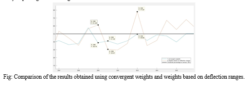
However, in the case of data number 302, the second approach proved to be more appropriate. This patient had values exceeding the accepted values by 4–5 hundred percent in several variables. The second method interpreted the results as a 77.97% of probability of cancer and labeled the person as positive, while the method with convergent weights labeled him as healthy, since the probability (49.69%) in this case did not exceed the threshold of 50%.

In conclusion, both approaches provided reliable results only in some cases. The convergent weights did not emphasize sufficiently the differences between healthy and potentially unhealthy patients and in many cases indicated an opposite diagnosis than working with the proportional weights. The weights based on deflection ranges were dependent on a few particular variables in an unbalanced way.

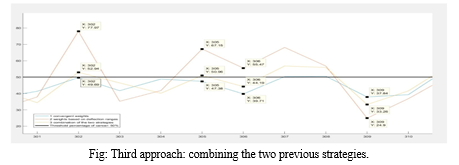
Misdiagnosing a healthy person as “at risk of having colorectal cancer” is called false positive, while labeling a patient with high risk of cancer as healthy is false negative diagnosis. Taking into consideration that fact that a computer aided diagnosis system should, in the first place, reduce the risk of cancer miss-rate and draw the attention of the doctor to any anomaly, the number of false negatives should be reduced to the maximum extent. Therefore, to avoid the huge differences in the order of magnitudes of the weights and reduce the number of false negatives, a third approach was imposed from the combination of the previous strategies. These “final” weights were numbers between 0.01 and 0.03, so convergent, but also expressing in their values the importance of each variable.

In Figure is shown the results given by these weights. There are two important behaviors to be observed. Firstly, that the final results represented by the yellow line are between the results given by the other two strategies, regardless of the nature of the diagnosis or the sign of difference between them. The second behavior of the final strategy can be examined in the case of data number 305 and 302. These records had results indicating that they had a chance of colorectal cancer, but the convergent weights (represented by the blue color in the figure) gave false negative results.

4. Normalizing the Continuous Response Variable

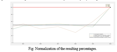
When determining the probability of cancer, it was crucial to ensure that the values ranged between 0 and 100%. Since the deviation of many variables from their healthy ranges often exceeded 100%, the calculated cancer risk could also surpass 100%. To address this, a two-step normalization process was implemented.

First, the maximum possible value for the cancer probability was calculated. A fictive patient, representing a 100% cancer probability, was created by assigning maximum possible values to all variables. The cancer probability for this worst-case scenario patient was then computed.

Second, with the worst-case scenario established, all results were normalized relative to this maximum percentage. This normalization involved dividing each patient's cancer probability by the worst-case probability. As shown in figure, this approach ensured that all three algorithms converged to 100% for the fictive patient, despite yielding different results for other patients.

Key roles in our scheme include the Dealer, responsible for generating and distributing shadow images and encryption keys to participants; Participants, who receive a shadow image and encryption key, encrypt it, and upload it to the blockchain; the Applicant, a participant intending to restore the secret image; and Agent Miners, network nodes responsible for computing polynomials in the encryption domain for image restoration.

B. Developing the Machine Learning Model

The primary goal of the research was to solve a binary classification problem. To train the model, a labeled response variable was necessary to represent the model's output in response to the input data. A person was considered unhealthy and suspected of having colorectal cancer if their probability of having a tumor exceeded 50%. In such cases, the response variable was set to 1; otherwise, it was set to 0. This threshold was determined based on expert consultation.

1. Training and Validation

After obtaining the predictors and the response variable, several models were trained using MATLAB®'s Classification Learner toolbox. This toolbox allows for model training with both k-fold cross-validation and holdout validation. Models were trained using two validation techniques, each with three different approaches. At the end of these six experiments, the best-performing models from each approach were compared.

2. K-Fold Cross Validation

The first validation technique used was k-fold cross-validation. Three different approaches were tested: 5-fold, 25-fold, and 50-fold cross-validation. Both accuracy and efficiency were considered when comparing the resulting models to identify the best performer.

3. 5-Fold Cross Validation

In the first approach, the dataset was divided into 5 folds, with k set to 5. The best-performing model using this approach was logistic regression, achieving an accuracy of 71.1% with a training time of 7.56 seconds. However, as seen in the confusion matrix in figure, the model had a relatively low number of false negatives (59) compared to false positives (201). Despite this, the false negative rate was 6.55%, which is unacceptably high for computer-aided cancer diagnosis systems.

C. Regression Problem Solved with Artificial Neural Networks

1. Reasoning of the Second Approach

For cancer detection software to be reliable, it should have an accuracy between 89% and 95% to provide experts with a dependable second opinion. The initial results from the Classification Learner toolbox showed that even the best-performing model—a linear discriminant model using 5% holdout validation—only achieved an accuracy of 77.8%. This level of accuracy is inadequate for a computer-aided cancer diagnosis (CAD) system, indicating that simply solving a classification problem might not yield sufficient results. This necessitated a different approach.

To improve the CAD diagnosis system, a change was made in the nature of the input data. Initially, the labeled dataset was used as input for constructing the machine learning models, resulting in both the input and output being binary variables. In the revised approach, continuous input data was used to avoid information loss from converting continuous to discrete variables. The percentage deviation from the healthy range for each input variable was considered in constructing the response variable.

A binary classification approach can be problematic because it doesn’t account for the nuanced reality of medical diagnosis. For instance, it is unrealistic to consider someone with a 49.9% probability of having cancer as healthy, while labeling someone with a 50.1% probability as unhealthy. This method can lead to a significant number of false negatives. Therefore, the classification problem was transformed into a regression problem to provide a more realistic diagnosis. The model now provides a continuous probability of cancer, displayed as a percentage on the user interface. While binary predictors were necessary for obtaining the continuous response, they were not used as inputs in the model construction and training.

Additionally, considering that deep neural networks perform better on large datasets than basic machine learning algorithms, the regression problem was tackled using MATLAB®'s Neural Network toolbox rather than the Regression Learner.

2. The Architecture of the Network

The performance of a deep learning algorithm heavily depends on the architecture and parameters of the neural network. To achieve the highest possible accuracy for the CAD system, 10 different network architectures were tested and their performance compared. This approach aligns with a similar study where several deep and shallow neural network models were compared to enhance the CAD system's sensitivity, specificity, and accuracy. In this study, 10 feedforward networks with backpropagation were trained, varying the number of layers and neurons across low, medium, and large configurations. The final network architecture was determined based on the performance of these nine initial networks. The performance function used was Mean Squared Error (MSE), and the Levenberg–Marquardt algorithm was chosen for training.

In addition to MSE, four other performance parameters were evaluated: the number of epochs, training time, gradient, and accuracy. The primary goal was to minimize MSE and maximize accuracy, with a secondary objective of minimizing training time and gradient. The data was divided into 60% for training and 20% each for testing and validation. Validation checks were set to six during training to prevent overfitting, limiting the number of iterations on the training dataset with the same performance function value.

The networks were trained on a computer with an i7 9700K CPU (4.7 GHz Turbo Boost) and 16 GB of DDR4 memory. It is important to note that the performance measures of the networks may vary depending on the hardware used for training.

3. Examination of the Networks

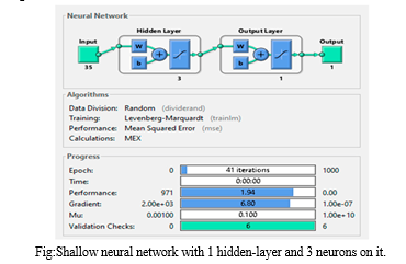
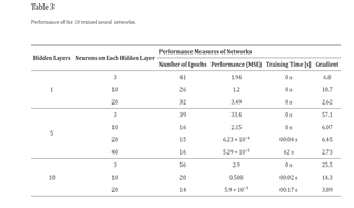
The first set of neural networks examined were shallow networks, each with a single hidden layer and varying neuron counts. The network with three neurons achieved an MSE of 1.94 after 41 iterations, with a training time of 0 seconds and a gradient of 6.8. The MSE nearly reached its minimum by the eighth epoch, and despite an increase in the test curve after the 24th epoch, no significant overfitting was observed. The network with ten neurons produced a similar MSE, also with a training time of 0 seconds, but the training stopped after 26 epochs and the gradient was higher at 10.7. The validation curve reached its minimum MSE at the 20th epoch, with the test curve showing a smaller MSE, indicating no overfitting. The network with twenty neurons had the highest MSE at 3.49 and reached its best performance after 26 iterations out of 32, with a gradient of 2.62. Across all shallow networks, the MSE remained within the 0-10 range.

The second set of networks were deep neural networks with five hidden layers, using the same neuron counts as the shallow networks. The network with three neurons per layer performed poorly, with an MSE ten times higher than any shallow network and a gradient of 57.1, though it did not exhibit overfitting or underfitting. The network with ten neurons per layer had an MSE of 2.15, a gradient of 6.07, and a training time of 0 seconds, but required only 16 iterations, fewer than the shallow networks, without affecting the training time. The best-performing model among the first nine ANNs was the deep network with five hidden layers and twenty neurons per layer, which had a significantly lower MSE of 0.000623, achieved in just 15 epochs with a training time of 4 seconds and an average gradient of 6.45. This network's MSE was ten times smaller than the second-best network (which had ten layers and twenty neurons per layer) and 50,000 times smaller than the worst-performing network (which had five layers and three

neurons).

The final three networks were deep networks with ten hidden layers and varying neuron counts. The network with three neurons per layer had an MSE comparable to the shallow networks, a gradient of 25.5, and the highest number of iterations at 56, with a training time of 0 seconds. Despite avoiding overfitting and underfitting, it provided mediocre results in minimizing the cost function. Increasing the neurons to ten per layer improved performance, with an MSE of 0.508 and a training time of 2 seconds after 20 epochs. However, the performance plot indicated significant overfitting after the tenth epoch, as the test curve increased sharply while the validation curve continued to descend, demonstrating that the model learned the noise from the training dataset.

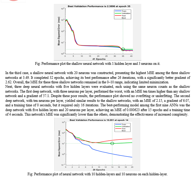
Three more deep networks with ten hidden layers and varying neuron counts were then evaluated. The network with three neurons per layer had an MSE comparable to the shallow networks, with a gradient of 25.5 and the highest number of iterations at 56, and a training time of 0 seconds. Despite avoiding overfitting and underfitting, it offered mediocre cost function minimization. Increasing the neurons to ten per layer improved performance, with an MSE of 0.508 and a training time of 2 seconds after 20 epochs. However, the performance plot indicated significant overfitting after the tenth epoch, as the test curve increased sharply while the validation curve continued to descend, suggesting the model learned the noise from the training dataset.

Based on insights gained from training the first nine networks, a 10th deep neural network was designed to maximize performance. This optimized structure was derived from two key observations: minimizing the MSE required a higher number of neurons compared to the number of hidden layers, and achieving minimal training time necessitated maintaining a medium number of hidden layers. Consequently, the 10th ANN was configured with five hidden layers, each containing 40 neurons.

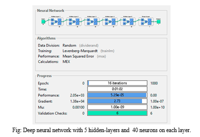
The training results of this final model validated the conclusions from earlier experiments. The high complexity of the network led to a training time exceeding one minute, despite the low number of epochs needed for completion. This network excelled in minimizing the MSE, achieving a value of 5.29 × 10−5, which was over ten times better than the best performing ANN from the previous experiments. Additionally, it recorded an impressive gradient of 2.73, the second smallest among all networks. The structure of this top-performing deep neural network is illustrated in the accompanying figure.

VII. RESULTS AND ANALYSIS

A. Classification Problem

After training various classification algorithms, the models were compared based on several performance metrics: accuracy, training time, percentage of false negatives, sensitivity, specificity, and precision.

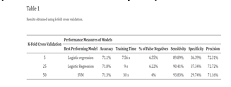
Upon evaluating the results using k-fold cross validation, the highest accuracy of 71.8%, specificity of 37.34%, and precision of 72.72% were achieved with the 25-fold cross validation using Logistic Regression. This model had a training time of 9 seconds, significantly less than other models achieving 71.3% accuracy from 50-fold cross validation. In terms of false negatives, the medium Gaussian SVM performed the best with only 4% false negatives among 900 records, which is 2.22% lower than the false negatives observed in the logistic regression models from both 25- and 50-fold cross validations.

Table 1 summarizes the results obtained from applying k-fold cross validation. The column labeled "% of false negatives" indicates the proportion of false negatives relative to the total samples in the validation dataset, which consists of 900 samples in this case. When comparing the outcomes from all three holdout validation techniques, the highest accuracy of 77.8%, sensitivity of 100%, specificity of 37.5%, and zero false negatives were achieved using 5% holdout validation with the linear discriminant model. Upon evaluating all six resulting models from both cross and holdout validation, it was determined that the linear discriminant model from 5% holdout validation performed the best.

Analyzing the average performance measures across the models, using k-fold cross validation resulted in models with an average accuracy of 71.4%, average training time of 15.52 seconds, and an average percentage of false negatives from the test dataset at 5.59%. The average sensitivity across the six models was 94.04%, specificity was 1.45%, and average precision was 71.71%.

In contrast, holdout validation techniques showed better results in the first four performance measures (see Table 2). The average accuracy of the best performing models was 72.8%, with an average training time of 4.55 seconds and a false negative rate of 2.12%. However, k-fold cross validation yielded better results in terms of specificity and precision. In conclusion, holdout validation demonstrated slightly superior performance compared to k-fold cross validation.

Our findings align with similar studies in the field. For instance, in [23], accuracies ranged between 66.9% and 74.51%, sensitivities between 49.36% and 66.82%, specificities between 80.42% and 80.97%, and precisions between 68.12% and 74.11%. Another method proposed by Blanes-Vidal et al. [22] achieved higher results with an accuracy above 96%, sensitivity of 97%, and specificity of 93%. Additionally, in colorectal cancer detection during colonoscopy [38], three models were compared, with accuracies ranging from 52.60% to 68.91%, sensitivities from 19.55% to 87.43%, and specificities from 42.47% to 90.55%.

Our study's outcomes closely mirror those reported in related research. For instance, accuracy, sensitivity, and specificity metrics varied across different studies. One notable study achieved accuracies ranging from moderate to high, demonstrating variability in sensitivity and specificity. Another study showcased superior performance, achieving high accuracy, sensitivity, and specificity metrics. In research focused on colorectal cancer detection during colonoscopy, various models yielded differing results, underscoring the challenge of consistently achieving robust diagnostic capabilities in this critical domain.

B. Regression Problem

After training all 10 neural networks, several key observations emerged regarding their performance. Contrary to expectations, increasing the complexity of the networks by adding more layers or neurons did not consistently improve performance. It was found that when the number of neurons was equal to or smaller than the number of hidden layers, the networks tended to perform poorly. Therefore, it was inferred that both the number of neurons and the number of hidden layers should ideally increase together to optimize performance. For instance, comparing the performance of a shallow neural network with three neurons in its hidden layer to that of deep neural networks with five layers and varying numbers of neurons (as detailed in Table 3) highlights this relationship.

Furthermore, the efficiency of gradient minimization was found to correlate closely with the number of neurons in the artificial neural network (ANN). Networks with a greater number of nodes in their hidden layers tended to achieve more efficient gradient minimization. Table 3 reveals an interesting correlation between the efficiency of cost function minimization and training time. The top-performing networks, which achieved the smallest Mean Squared Error (MSE), typically required seconds to train, ranging from 2 to 62 seconds. In contrast, the remaining networks showed negligible training times (0 seconds), indicating minimal or no perceptible training effort. Comparing the MSE achieved by the best-performing model in this study with results reported , it is evident that our MSE of 5.29 × 10−5 is significantly lower than the MSE of 0.01 achieved , despite their 2000 epochs of training. This underscores the efficacy of our approach in achieving highly accurate predictions.

The best-performing deep neural network achieved an accuracy of 99.106%, affirming that the developed Computer-Aided Diagnosis (CAD) system meets the criteria for a reliable and intelligent cancer diagnostic tool. When compared with other state-of-the-art diagnostic systems documented, our system demonstrates competitive accuracy, reflecting a significant advancement in computer-aided diagnosis.

Conclusion

Based on the outcomes derived from addressing the binary classification problem using conventional machine learning algorithms, achieving an accuracy of only 77.8% falls short of the requisite reliability for a cancer detection software intended to provide expert second opinions. Additionally, for such software to offer dependable diagnoses, it\'s imperative that the output provides a continuous percentage-based response rather than a discrete variable to mitigate the risk of misdiagnosis. Consequently, the approach was redirected towards transforming the binary classification problem into a regression problem. To address this regression problem effectively, artificial neural networks (ANNs) were explored as a more suitable machine learning technique. Ten different network architectures were trained, each varying in its ability to minimize the cost function, specifically the mean squared error (MSE). The most successful ANNs included a deep neural network featuring five hidden layers, with each layer comprising 40 neurons. This optimized configuration significantly reduced the MSE to the order of 10?5 and achieved an impressive accuracy of 99.106%. In summary, deep neural networks have proven to be more robust and effective in colorectal cancer detection compared to traditional machine learning approaches. Optimal neural network structures should prioritize numerous neurons distributed across multiple hidden layers, ensuring both high performance and efficiency in terms of training duration. The innovative dataset structure employed in this study introduces a novel approach to non-invasive colorectal cancer diagnosis. By combining numerical data from blood and urine analyses with qualitative data, the diagnostic process becomes more comprehensive and precise. Future advancements aim to integrate image processing capabilities into this intelligent colorectal cancer detection software, thereby enabling the detection of cancerous features in colonoscopy images.

References

[1] Keum N., Giovannucci E. Global burden of colorectal cancer: emerging trends, risk factors and prevention strategies. Nat. Rev. Gastroenterol. Hepatol. 2019;12:713–732. doi: 10.1038/s41575-019-0189-8. [PubMed] [CrossRef] [Google Scholar] [2] Rwala P., Sunkara T., Barsouk A. Epidemiology of colorectal cancer: incidence, mortality, survival, and risk factors. Prz. Gastroenterol. 2019;14:89–103. doi: 10.5114/pg.2018.81072. [PMC free article] [PubMed] [CrossRef] [Google Scholar] [3] Rampun A., Wang H., Scotney B., Morrow P., Zwiggelaar R. Classification of mammographic microcalcification clusters with machine learning confidence levels; Proceedings of the 14th International Workshop on Breast Imaging; Atlanta, GA, USA. 8–11 July 2018. [Google Scholar] [4] Goel N., Yadav A., Singh B.M. Medical image processing: A review; Proceedings of the IEEE Second International Innovative Applications of Computational Intelligence on Power, Energy and Controls with Their Impact on Humanity (CIPECH); Ghaziabad, India. 18–19 November 2016. [Google Scholar] [5] Ameling S., Wirth S., Paulus D., Lacey G., Vilarino F. Texture-Based Polyp Detection in Colonoscopy. In: Meinzer H.P., Deserno T.M., Handels H., Tolxdorff T., editors. Bildverarbeitung für die Medizin 2009: Informatik aktuell. Springer; Berlin, Heidelberg: 2009. pp. 346–350. [Google Scholar] [6] Ali H., Sharif M., Yasmin M., Rehmani M.H., Riaz F. A survey of feature extraction and fusion of deep learning for detection of abnormalities in video endoscopy of gastrointestinal-tract. Artif. Intell. Rev. 2020;53:2635–2707. doi: 10.1007/s10462-019-09743-2. [CrossRef] [Google Scholar] [7] Alagappan M., Brown J.R.G., Mori Y., Berzin T.M. Artificial intelligence in gastrointestinal endoscopy: The future is almost here. World J. Gastrointest. Endosc. 2018;10:239–249. doi: 10.4253/wjge.v10.i10.239. [PMC free article] [PubMed] [CrossRef] [Google Scholar] [8] Gheorghe G., Bungau S., Ilie M., Behl T., Vesa C.M., Brisc C., Bacalbasa N., Turi V., Costache R.S., Diaconu C.C. Early Diagnosis of Pancreatic Cancer: The Key for Survival. Diagnostics. 2020;10:869. doi: 10.3390/diagnostics10110869. [PMC free article] [PubMed] [CrossRef] [Google Scholar] [9] Bel’skaya L.V., Sarf E.A., Shalygin S.P., Postnova T.V., Kosenok V.K. Identification of salivary volatile organic compounds as potential markers of stomach and colorectal cancer: A pilot study. J. Oral Biosci. 2020;62:212–221. doi: 10.1016/j.job.2020.05.002. [PubMed] [CrossRef] [Google Scholar] [10] Pang S.-W., Awi N.J., Armon S., Lim W.-D., Low J.-H., Peh K.-B., Peh S.-C., Teow S.-Y. Current Update of Laboratory Molecular Diagnostics Advancement in Management of Colorectal Cancer (CRC) Diagnostics. 2020;10:9. doi: 10.3390/diagnostics10010009. [PMC free article] [PubMed] [CrossRef] [Google Scholar] [11] Ludvigsen M., Thorlacius-Ussing L., Vorum H., Moyer M.P., Stender M.T., Thorlacius-Ussing O., Honoré B. Proteomic Characterization of Colorectal Cancer Cells versus Normal-Derived Colon Mucosa Cells: Approaching Identification of Novel Diagnostic Protein Biomarkers in Colorectal Cancer. Int. J. Mol. Sci. 2020;21:3466. doi: 10.3390/ijms21103466. [PMC free article] [PubMed] [CrossRef] [Google Scholar] [12] Jaberie H., Hosseini S.V., Naghibalhossaini F. Evaluation of Alpha 1-Antitrypsin for the Early Diagnosis of Colorectal Cancer. Pathol. Oncol. Res. 2020;26:1165–1173. doi: 10.1007/s12253-019-00679-0. [PubMed] [CrossRef] [Google Scholar] [13] Xu W., Zhou G., Wang H., Liu Y., Chen B., Chen W., Lin C., Wu S., Gong A., Xu M. Circulating lncRNA SNHG11 as a novel biomarker for early diagnosis and prognosis of colorectal cancer. Int. J. Cancer. 2019;146:2901–2912. doi: 10.1002/ijc.32747. [PubMed] [CrossRef] [Google Scholar] [14] Lin J., Cai D., Li W., Yu T., Mao H., Jiang S., Xiao B. Plasma circular RNA panel acts as a novel diagnostic biomarker for colorectal cancer. Clin. Biochem. 2019;74:60–68. doi: 10.1016/j.clinbiochem.2019.10.012. [PubMed] [CrossRef] [Google Scholar] [15] Toiyama Y., Okugawa Y., Goel A. DNA methylation and microRNA biomarkers for noninvasive detection of gastric and colorectal cancer. Biochem. Biophys. Res. Commun. 2014;455:43–57. doi: 10.1016/j.bbrc.2014.08.001. [PMC free article] [PubMed] [CrossRef] [Google Scholar]

Copyright

Copyright © 2024 Shashank R R, Indudhara S, Aditya A Navale. This is an open access article distributed under the Creative Commons Attribution License, which permits unrestricted use, distribution, and reproduction in any medium, provided the original work is properly cited.