Global Weight Optimization on Artificial Neural Network for Optimizing Crop Yield Prediction Using Genetic Algorithm

Abstract

Accurate crop yield prediction is a complex and intricate task that encompasses a multitude of factors and variables, rendering it arduous to establish a dependable mathematical model. Conventional machine learning (ML) models for crop yield prediction have surpassed their efficacy. This research endeavour sought to enhance crop yield prediction accuracy by hybridizing a neuro-genetic model utilizing statistical data amassed over a 35-year period from various pertinent agricultural departments in Tamil Nadu, India, including the Statistical, Agricultural, and Meteorological Departments. This research delved into analyzing and identifying the optimal weight configuration for the artificial neural network (ANN) to bolster accuracy with the assistance of genetic algorithms (GA). Seventy-five percent of the data was employed to train the model, while the remaining 25% was utilized for model testing. To gauge the performance of this research work, 5-fold cross-validation was implemented. RMSE, MAE, and Adj R2 were employed to evaluate the performance and contrast the performance of the neuro-genetic model with the conventional ANN. The neuro-genetic model exhibited superior accuracy compared to the conventional ANN.

Introduction

I. INTRODUCTION

Ensuring food security is paramount to achieving the Sustainable Development Goals (SDGs), and paddy, a staple crop in Asia and a significant global food source, plays a critical role in this endeavor (Bin Rahman A. N. M., & Zhang J., 2023). Economic models predict a substantial increase in food demand by 2050, ranging from 59% to 98% (Hugo Valin et al., 2014; OECD-FAO Agricultural Outlook 2021-2030, 2021), necessitating a substantial expansion in paddy production. Several factors, including rainfall, temperature, and soil type, significantly impact crop yield (Maya Gopal P.S., Bhargavi R., 2019a). Accurate yield prediction models are crucial for assisting planning departments in making informed decisions to optimize agricultural practices and ensure food security. Machine learning methods applied to multi-farm datasets have demonstrated the potential for accurate yield forecasting (Filippi P. et al., 2019). Pre-harvest yield predictions are essential for various stakeholders, including the farmers, to optimize management practices and national authorities to forecast food grain imports and exports. The precise prediction of yield is essential for maximizing paddy yield within the constraints of limited land resources. The lack of a benchmark dataset for agricultural research poses a challenge in evaluating and comparing the performance of different prediction models. These datasets are primarily obtained from local authorities and producers' associations through field observations and expert surveys, which may introduce biases and inaccuracies.

Machine learning algorithms have become a cornerstone in crop yield prediction, with Artificial Neural Networks (ANNs) taking center stage. Thawornwong S. & Enke D. (2004) and Agrawal, J.D. & Deo, M.C. (2004) give the adaptive nature of variables in improving forecasting accuracy through modified neural network models, highlighting the intricate interplay between variables. ANNs possess several strengths, including their ability to learn directly from data without parameter estimation, statistical properties, and the capacity to approximate any continuous nonlinear function. However, ANNs have their limitations, facing challenges such as low convergence and entrapment in local minima. Researchers have proposed optimizing ANNs with other algorithms to address these issues and enhance their performance. The training of neural networks is a complicated and time-consuming process. In this context, appropriate fitness functions are employed as ANN parameters. Xin Yao and Yong Liu (1997) meticulously analyzed the behavior of ANNs and concluded that weight optimization is a critical aspect of ANN performance.

The genuine function to be optimized contains numerous local minima. Therefore, researchers have used global search algorithms to train neural networks instead of traditional local search algorithms. Global optimization algorithms are a class of algorithms that seek to avoid getting trapped in local minimums. Genetic algorithms are the most common evolutionary algorithm used to train neural networks. This methodology has proven to be effective in addressing a range of engineering challenges. The back-propagation algorithm and genetic algorithms (GAs) can enhance the performance of ANNs. Researchers such as Branke J. (1995) and Xin Yao (1999) have proposed and compared various schemes for integrating GAs and ANNs, primarily focused on optimizing network weights or identifying optimal network topologies. The present study seeks to enhance the accuracy of crop yield prediction by utilizing a genetic algorithm to determine the optimal initial weights for an artificial neural network. In this context, this paper aims to introduce a novel approach to crop modeling that incorporates a genetic model to improve the precision of crop yield predictions. The back-propagation algorithm's susceptibility to becoming trapped in local minima and its high dependence on initial weights necessitates using a GA to optimize ANN weights.

To effectively predict crop yield, this research employs the back-propagation ANN (BPNN) algorithm, a multilayer network that quantifies the influence of each variable using weights. The input layer consists of a neuron for each variable, while the output layer produces the estimated values of the inputs. The study seeks to optimize the BPNN's initial weights using a genetic algorithm (GA) to enhance yield prediction accuracy. The GA generates a random population of chromosomes representing the neuro-genetic model parameters. These chromosomes undergo evolutionary operations and selection for reproduction. Each chromosome's fitness is evaluated to determine which chromosomes survive for selection in subsequent generations. The GA iteratively evolves until the best fitness value in the population cannot be improved, yielding the optimal parameters of the neuro-genetic model as the best-converged solution. The study also investigates the neuro-genetic model's sensitivity to parameter settings and utilizes initial trials to identify optimal parameter settings.

II. WORKFLOW

The research work has been divided into 8 procedures. Figure 1 illustrates the workflow of the research. The subsequent subsections of the paper discuss the workflow in detail.

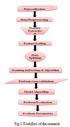
A. Data Collection

The initial step in the research process involved data collection, following the selection of the research field. However, prior to data collection, it was crucial to identify the data types necessary for the successful implementation of the proposed model. An extensive literature review was conducted to determine the factors influencing crop production and resource utilization. Drawing from various research works on literature and agricultural practices, the relevant features were selected for the research. Notably, the Indian agricultural sector remains unorganized, with farmers relying on their traditional knowledge and small landholdings for cultivation. The Ministry of Agriculture provides general guidelines for the region, while various ministries maintain separate agricultural data repositories. Consequently, the required data was not readily available in any existing open databases or datasets. Additionally, the available online data, primarily handwritten and scanned, was not machine-readable and hence unsuitable for use in the proposed model. Therefore, primary research was deemed necessary to gather the required data. Data collection efforts involved collaboration with the Statistical, Agricultural, and Meteorological Departments of the Tamil Nadu state government. From these departments, district-wise statistical data for paddy crops was collected for three decades (1986-2022), encompassing irrigation, planting area, fertilizer usage, number of seeds used, and meteorological data related to temperature, rainfall, and solar radiation.

B. Data Pre-processing

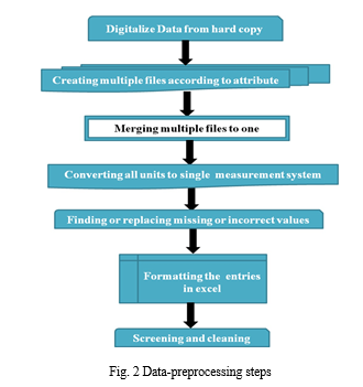
The subsequent crucial step in the workflow involved data preprocessing, a process aimed at rendering the data comprehensible to the machine learning model. Figure 2 illustrates the stages involved in data preprocessing. This step entailed identifying, eliminating, or replacing unreliable, incomplete, or irrelevant data. However, in the present study, data digitization from hard copies, merging multiple data files from various ministries into a single file, converting all data to a consistent unit system, identifying missing values or entries, formatting entries, eliminating redundant values, and data cleaning were necessary due to the non-standard data format. Some entries were missing, and a significant portion of the data existed in hard copies. Additionally, due to the data's collection from multiple sources, conflicting values were present in some entries. In such instances, determining the more reliable values was essential. Moreover, redundant entries were prevalent and required filtering. During this process, unnecessary entries in the collected data were also filtered out, and the data needed to be converted from multiple formats into a consistent unit system. Following the screening and cleaning processes, data formatting was necessary, and the CSV file was subsequently utilized in the model.

C. Feature Normalization (Scaling)

The scale of attributes significantly impacts the effectiveness of data mining techniques. Improper scaling can lead to modeling errors, as attributes with larger scales tend to receive undue emphasis during the modeling process. This issue can be effectively addressed by normalizing the attributes to a specified range. Attribute normalization involves standardizing the ranges of independent variables or features, a technique commonly known as data normalization. This process was implemented during the data preprocessing stage. A noteworthy aspect of this dataset is that each attribute is accompanied by its respective measurement units. In the present study, the attributes were scaled to fall within the value of 0 to 1. The accurate prediction can be obtained by rescaling the dataset using the equation

where X’ is the new scaled value, X is the variable’s value, min(X) is the variable’s lower limit value and max(X) is the variable’s upper limit value.

D. Feature Selection

Feature selection is a crucial step in machine learning, aiming to identify and eliminate irrelevant or redundant features from a dataset, thereby reducing its dimensionality and computational complexity. This process is particularly important to prevent overfitting, a phenomenon where a model performs well on the training data but poorly on unseen data. Overfitting can occur when a model learns from noise and irrelevant features, leading to poor generalization ability. However, in the context of the current study, feature selection was not employed as the dataset was manually constructed, meticulously eliminating unnecessary variables from the outset. This careful curation ensured that the dataset contained only relevant features, effectively mitigating the risk of overfitting and enhancing the model's generalizability.

E. Data Splitting

Data splitting is an integral component of supervised machine learning and data science applications, as it directly influences the accuracy of the model's predictions. In this study, the collected data was initially divided into two subsets for training and testing purposes. This initial data splitting aimed to balance the number of rows across all attributes, mitigating any potential anomalies that could affect the model's performance. Additionally, eliminating unused rows reduced processing time and enabled the algorithm to operate efficiently on less powerful computing resources. The standard 80:20 ratio was initially adopted, with 80% of the data used for training and 20% for testing. This distribution was consistently applied throughout the research process. Subsequently, the data was further split into a 75:25 ratio, and the same process was followed to achieve higher accuracy. This refined ratio was ultimately utilized in the final model.

F. Training and Testing of the Algorithm

As previously stated, the data was subdivided into two segments. One portion of the partitioned data was utilized to train the algorithm, while the remaining portion was employed to test its performance. Following the successful training and evaluation of the algorithm using this split dataset, a comparable procedure was implemented for all of the algorithms that were employed.

G. Performing Cross-Validation

Cross-validation, a statistical resampling method, is employed to assess the validity and generalizability of a model by comparing its predictions on a portion of the data (test set) to its performance on the remaining portion (training set). This process helps to identify whether the model is adequately fitted or overfitted to the data. To determine the mean cross-validation score, this method has been applied to multiple train-test splits. Cross-validation, with its systematic approach, overcomes the issues associated with random subsampling. Traditionally, the holdout set is randomly selected multiple times. An alternative approach in the cross-validation process involves dividing the dataset into k equal-sized subsets, or folds, before training. Subsequently, k models are trained using one subset as the test set and the remaining k-1 subsets as the training set. This ensures that each subset is used as a test set at least once, maximizing the utilization of all data points. In this process, each data point is used for testing once and for training k-1 times. In the present research work, 5-fold cross-validation was performed to assess the model's performance.

H. Performance Evaluation of Models

The performance of each model is assessed using well-established metrics such as the Root Mean Square Error (RMSE), the Mean Absolute Error (MAE), and the correlation coefficient (R).

The RMSE quantifies the difference between the estimated and actual values, with larger values indicating greater discrepancies. However, it is sensitive to outliers, meaning that extreme values can disproportionately influence the overall error measurement. The R-value, on the other hand, reflects the strength of the linear relationship between the estimated and actual values. A higher R-value indicates a stronger linear association, suggesting that the model effectively captures the underlying pattern in the data. The MAE, representing the average magnitude of the errors, provides a measure of the overall prediction accuracy. Once the features are incorporated into the Multiple Linear Regression (MLR) model, its accuracy is evaluated and interpreted by calculating the Rˆ2 value.

I. Generate Final Prediction

The final prediction of the model was generated by running the best performing algorithm on the selected parameters.

J. Fitting

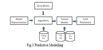
The most crucial part of the model was to fit the data. The machine-learned from the train set was used later while predicting the test set as shown in Figure 3.

K. Accuracy

To assess the performance of the chosen algorithms, various accuracy-checking methods were implemented tailored to the specific requirements of each algorithm. In the case of artificial neural networks (ANNs), while an accuracy-checking method was invoked, the overall accuracy was determined by averaging the accuracy values across all epochs. This evaluation of accuracy is essential for assessing the viability of the algorithms employed and the research itself. If all algorithms consistently yield very low accuracy, it would indicate that the proposed method as a whole is not suitable for further investigation. Conversely, if some algorithms exhibit low accuracy while others achieve high accuracy, it suggests that the low-performing algorithms are not efficient within the specific model, while the others demonstrate promise. Notably, all algorithms employed in this study demonstrated reasonably high accuracy. An effective model is one that consistently produces predictions that closely align with the actual values of the test data, outperforming the performance of other models.

L. Comparing Model

The existence of a single, universally superior classification technique is an elusive concept, as no single approach can excel in all possible learning tasks (Schaffer, 1994). This inherent limitation has led to the development of multiple models employing diverse techniques and configurations during data mining endeavors. The creation of these models necessitates a structured approach to comparing and selecting the most effective one. The question of how to best compare classifiers has been a subject of extensive research, resulting in a plethora of available evaluation methods.

M. Features used for Analysis

This research has identified several features, parameters, or attributes that are crucial for agricultural production. These factors have a significant impact on agricultural output in the selected regions each year. The availability of data is the primary determinant of these attributes or parameters. The study utilized two distinct sets of statistical data: statistical and agricultural data for paddy production, along with weather data for the respective years. The collected two data sets were combined into a single data set. Table describes the dataset.

Table 1 Description of the dataset

Table 1 presents the parameters that are employed to assess paddy crop yield in the study area. The data indicate that the region experiences a moderate climate, devoid of extreme weather conditions. The sub-datasets within the agricultural production data provide detailed information regarding planting and irrigation areas, fertilizer usage, and irrigation practices. Climatic variables such as solar radiation, maximum and minimum temperatures, and rainfall are captured in the weather dataset. Each instance of the dataset invariably contains crop specifics, including the total cultivated area, annual production, and annual weather observations. The final dataset encompasses 745 instances with 16 documented features spanning a three-decade period, from 1986 to 2022. Notably, the 16 features considered include cultivation area in hectares, canal length in meters, number of tanks and open wells, total production in tons, rainfall in millimeters, maximum, minimum, and average temperatures, solar radiation, seed quantity used, nitrogen, phosphorus, and potassium applied to the soil in kilograms, and yield in tons per hectare.

III. MATERIALS AND METHODS

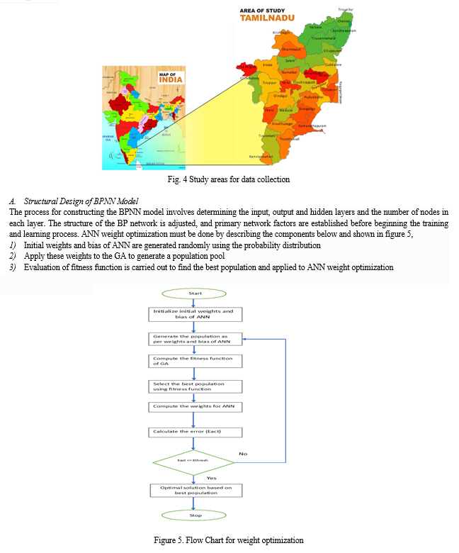
This study employed a dataset encompassing 35 years of paddy crop yield data from the State of Tamil Nadu, a southern Indian state situated within the tropical zone. Data acquisition encompassed various sources, including the Meteorological Department of India, the Tamil Nadu Department of Agriculture, and the Tamil Nadu Department of Statistics. The investigation incorporated a range of features, including planting area, number of tanks, number of tube wells and open wells utilized for irrigation, canal length for irrigation purposes, quantities of nitrogen, phosphorus, and potash fertilizers consumed, seed quantity allocated to the planting area, cumulative rainfall, cumulative global solar radiation, maximum, average, and minimum temperatures. To enhance prediction accuracy, the gathered data underwent a cleaning process and rescaling to a range spanning 0 to 1. Following are the GPS coordinates of the study areas: 11°7 37.6428 N and 78°39 24.8076 E and elevation are 138 m. Figure 4 depicts the study areas for data collection.

Training continues until the network becomes stable, the output meets the specified error requirements, or the maximum number of training repetitions is reached. Ki-Young Lee, et.al (2017) compared the artificial neural networks of linear learning and deep learning of machine learning and investigated the solution of the overfitting problem through artificial neural networks. Pan F., et.al (2020) introduced BPNN into the clone detection to improve the ability of dealing with multidimensional input. The trained neural network is evaluated using a test data set, and if it meets the specified accuracy, it has deterministic significance. The proposed methodology for developing the neuro-genetic model is presented in pseudo-code.

B. Pseudo code for Neuro Genetic Algorithm

1. Set all input and target data for the neural network.
2. Initialize weights and bias.
3. Transfer the weights to the genetic algorithm population.
4. Set population size (Ps)-20, Mutation (Mr)- 0.1, Crossover rate (Cr) = 0.03.(This is found after trial and error).
5. Incorporate fitness function:
6. Fitness =;
7. Stop the function when reaching the average tolerance rate of the fitness function.
8. Find the best performance value and the generated population.
9. Retransfer the population to reinitialized weights and reconstruct the neural network.
10. End the neural network.
11. Repeat from step 1 till reaching the optimized solution.

C. Parameters Setting for Training the Neural Network

This study utilizes the Neural Network Fitting Tool GUI (nnstool) available in MATLAB 7.6.0 to analyze the data using an Artificial Feed-Forward Neural Network (ANN) with back-propagation principles. The back-propagation algorithm, a common optimization technique in ANNs, is employed to predict crop yield.

To ensure a robust prediction model, 75% of the randomly selected data is utilized for training, while the remaining 25% is reserved for testing. The ANN architecture adopts a 5-3-1 configuration, with five input features extracted from Maya Gopal P.S. and Bhargavi R. (2019c).

These features include area in hectares, canal length, open well, tank, and maximum temperature, all of which are deemed relevant for crop yield prediction. To enhance the prediction accuracy, the input values of these features are rescaled to lie within the range of 0 and 1.

The ANN tool is employed to generate random initial weights, which serve as the initial population for the genetic algorithm. This algorithm is implemented with 21 chromosomes, and 200 generations with different populations are generated to obtain the optimal initial weights. The minimum fitness value falls within this range, ensuring the effectiveness of the optimization process. The randomly generated initial weights encompass three sets of weights for the three hidden neurons, three neurons in the subsequent layer, and three for the final neuron.

These weights are organized into five sets, with the first set of five corresponding to the first neuron in the hidden layer, the second set of five to the next neuron, and the third set of five to the last neuron.

The Genetic Algorithm (GA) relies on several critical parameters for successful implementation, including population size, mutation rate, and crossover rate.

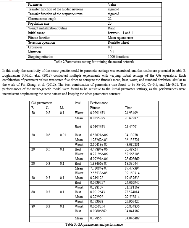
These parameters are interrelated, and determining the optimal values for them is typically done through trial and error due to the lack of defined rules for their selection. The optimal parameter values for successful GA implementation are crucial, as shown in Table 2.

This table presents the GA parameters that have a significant impact on performance, along with performance indicators evaluated for various initial parameter settings. Finding the optimal initial weights was challenging due to concerns about overfitting in neural networks and the limited search space of genetic algorithms. Moreover, the use of genetic algorithms should be based on the performance of neural networks on testing datasets rather than solely on the minimal square error in modeling datasets.

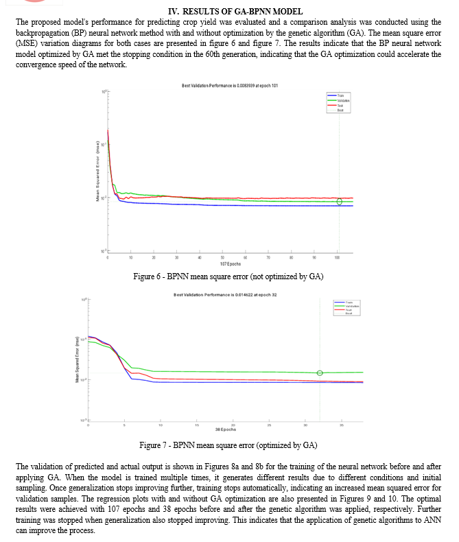
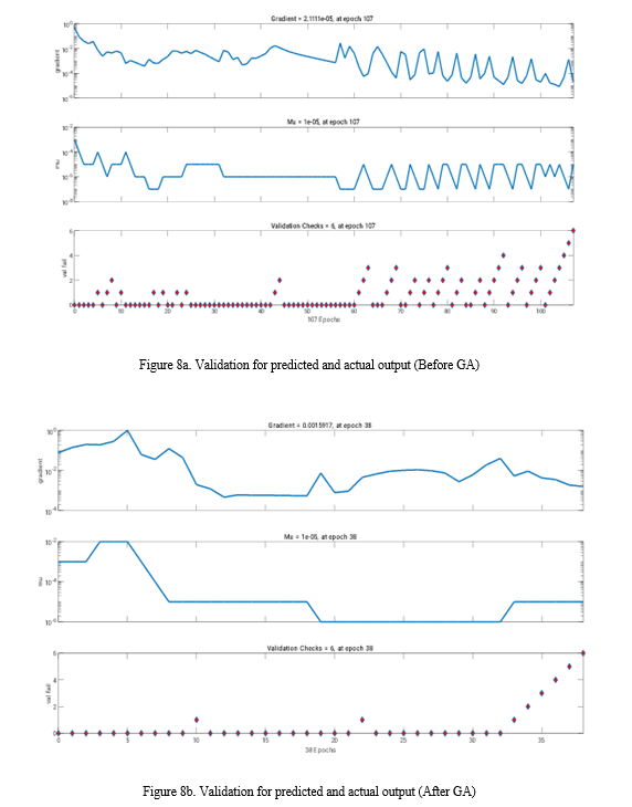
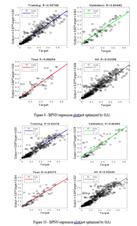
V. MODEL COMPARISON

The average assessment accuracy of the optimized BPNN model was 93.65%, while the average assessment accuracy of the GA-BPNN algorithm was 97.83%, demonstrating the superior performance of the GA-BPNN algorithm. This enhanced assessment accuracy is attributed to the optimization of the BP neural network's weights through the application of a genetic algorithm based on adaptive mutation. While this optimization strategy leads to more accurate and scientifically sound crop yield predictions, it also increases the computational time due to the additional genetic operations of coding, decoding, crossover, and mutation.

The correlation coefficient R2, which is a value that indicates the degree of a relationship, is measured to assess the performance of the ANN model and neuro-genetic model. The R2 value for the correlation between the ANN model and that predicted by the neuro-genetic model was computed to show the network's performance and is presented in Table 4. The results also showed a significant strong positive correlation between the crop yield predicted by the neuro-genetic and ANN models.

Table 4 Performance of the ANN and neurogenetic algorithm

VI. ACKNOWLEDGMENTS

The authors gratefully acknowledge the Statistical Department and Agricultural Department of the State Government of Tamil Nadu and the Meteorological Department in India for the statistical data for agrarian purposes.

Conclusion

In this research, a novel Neuro Genetic (NG) model is proposed and implemented for accurate crop yield prediction. The proposed model employs a Genetic Algorithm (GA) to initialize the weights of the artificial neural network (ANN), followed by back-propagation training to determine the true global minimum of the error function. The prediction accuracy is evaluated using standard performance metrics and compared to those of conventional ANN and neurogenetic models. The results demonstrate that the proposed NG model outperforms conventional ANNs in terms of prediction accuracy on the same agricultural dataset. These findings highlight the effectiveness of GA as an automated approach to ANN architecture design.

References

[1] Agrawal, JD & Deo, M.C. (2004). Wave parameter estimation using neural network. Mar. Struct. 17, 536–550. [2] Basso B., Liu L. (2019), Chapter four - seasonal crop yield forecast: methods, applications, and accuracies Adv. Agron., 154, pp. 201-255 [3] Bin Rahman A. N. M., & Zhang J. (2023). Trends in rice research: 2030 and beyond. Food and Energy Security, 12, e390. [4] Branke J. (1995), “Evolutionary algorithms for neural network design and training,” Univ. Karlsruhe, Inst. AIFB, Karlsruhe, Germany, Tech. Rep.322. [5] Drummond S.T., Sudduth K.A., Joshi A., Birrell S.J., Kitchen NR (2003). Statistical and neural methods for site-specific yield prediction. Trans. ASAE 46, 5–14. [6] Fei Zheng, Xianju Zhou, Changjong Moon, Hongbing Wang (2012) Regulation of brain-derived neurotrophic factor expression in neurons. Int. J Physiol Pathophysiol Pharmacol;4(4):188-200. [7] Filippi P., Jones E.J., Wimalathunge N.S., Somarathna PDSN, Pozza L.E., Ugbaje S.U., Jephcott T.G., Paterson S.E., Whelan B.M., Bishop T.F.A. (2019). An approach to forecast grain crop yield using multi-layered, multi-farm data sets and machine learning, Precis. Agric., 20, pp. 1015-1029 [8] Hugo Valin, Ronald D. Sands, Dominique van der Mensbrugghe, Gerald C. Nelson, Helal Ahammad, Elodie Blanc, Benjamin Bodirsky, Shinichiro Fujimori, Tomoko Hasegawa, Petr Havlik, Edwina Heyhoe, Page Kyle, Daniel Mason-D\'Croz, Sergey Paltsev, Susanne Rolinski, Andrzej Tabeau, Hans van Meijl, Martin von Lampe, Dirk Willenbockel (2014). The future of food demand: understanding differences in global economic models. Agric. Econ. 45, 51–67. [9] Hugo Valin, Ronald D. Sands, Dominique van der Mensbrugghe, Gerald C. Nelson, Helal Ahammad, Elodie Blanc, Benjamin Bodirsky, Shinichiro Fujimori, Tomoko Hasegawa, Petr Havlik, Edwina Heyhoe, Page Kyle, Daniel Mason-D\'Croz, Sergey Paltsev, Susanne Rolinski, Andrzej Tabeau, Hans van Meijl, Martin von Lampe, Dirk Willenbockel, (2014). The future of food demand: understanding differences in global economic models. Agric. Econ. 45, 51–67. [10] Ji B., Sun Y., Yang S. and Wan J. (2007). Artificial neural networks for rice yield prediction in mountainous regions. J. Agri. Sci. 145, 249–261. [11] Ki-Young Lee, Kyu-Ho Kim, Jeong-Jin Kang, Sung-Jai Choi,Yong-Soon Im,Young-Dae Lee, Yun-Sik Lim (2017), “Comparison and analysis of linear regression & artificial neural network,” International Journal of Applied Engineering Research, vol. 12, no. 20, pp. 9820–9825,. [12] Loghmanian S.M.R., Jamaluddin H., Ahmad R., Yusof R., Khalid M. (2012), Structure optimization of neural network for dynamic system modeling using multi-objective genetic algorithm, Neural Comput. Appl., 21 (6), pp. 1281-1295 [13] Lu Xing, Liheng Li, Jiakang Gong, Chen Ren, Jiangyan Liu, Huanxin Chen (2018). Daily soil temperatures predictions for various climates in united-states using data-driven model. Energy 160, 430–440. [14] Maya Gopal P.S., Bhargavi R. (2019a). \"A novel approach for efficient crop yield prediction, Computers and Electronics in Agriculture\", Volume 165, 104968 [15] Maya Gopal P. S. & Bhargavi R. (2019b) Performance Evaluation of Best Feature Subsets for Crop Yield Prediction Using Machine Learning Algorithms, Applied Artificial Intelligence, 33:7, 621-642, [16] Maya Gopal P.S. and Bhargavi R. (2019c) \"Selection of Important Features for Optimizing Crop Yield Prediction.\" IJAEIS vol.10, no.3 : pp.54-71. [17] OECD-FAO. (2021). OECD-FAO Agricultural Outlook 2021-2030. OECD Publishing. [18] Pan F., Wen H., Gao X., Pu H., and Pang Z. (2020), \"Clone detection based on BPNN and physical layer reputation for industrial wireless CPS,\" IEEE Transactions on Industrial Informatics, vol. 17, no. 5, pp. 3693–3702. [19] Paudel D., Boogaard H., De Wit A.J.W., Van Der Velde M., Claverie M., Nisini L., Janssen S., Osinga S., Athanasiadis I.N. (2022). Machine learning for regional crop yield forecasting in Europe Field Crops Res., 276 [20] Thawornwong S. & Enke D. (2004). The adaptive selection of financial and economic variables for use with artificial neural networks. Neurocomputing 56, 205–232. [21] Wallach D., Makowski D., Jones J.W., Brun F. (2019), Working with Dynamic Crop Models: Methods, Tools and Examples for Agriculture and Environment (Third. ed.), Academic Press, London, U.K [22] Xin Yao & Yong Liu (1997), “A new evolutionary system for evolving artificial neural networks,” IEEE Trans. Neural Netw., vol. 8, no. 3, pp. 694–713. [23] Xin Yao (1999), “Evolving artificial neural networks,” Proc. IEEE, vol. 87, no.9, pp. 1423–1447.

Copyright

Copyright © 2024 Parameswaran Sulochana Maya Gopal, Thangappan Sasikala . This is an open access article distributed under the Creative Commons Attribution License, which permits unrestricted use, distribution, and reproduction in any medium, provided the original work is properly cited.