A Comparative Examination of Machine Learning Algorithms for Predicting Cardiovascular Disease

Abstract

Over the previous few years, India’s heart disease incidence has varied between 1.2% and 13.2% in urban areas and 1.6% and 7.4% in rural areas. India would probably have more CVD deaths in 2020 which is 4.77 million compared to 2.26 million in 1990. Worldwide, 200 million individuals are estimated to be affected by heart disease. Heart disease affects over 110 million men and 80 million women globally. This study explores the use of machine learning (ML) with various models and data to predict cardiovascular illness with the goal of improving accuracy. Clinician parameters, lifestyle indicators, and demographic data are used to train and assess an assortment of machine learning methods, including Logistic Regression, Support Vector Machines, Random Forests, Decision Trees, and Naive Bayes.

Introduction

I. INTRODUCTION

Cardiovascular disease is a global health problem with a major impact on global mortality and morbidity. Its com- plexity, involving various cardiovascular conditions, presents challenges for healthcare systems. Early and precise prediction of heart disease is crucial for effective prevention and timely interventions. Traditional diagnosis relies on clinical factors and invasive procedures. However, Machine Learning (ML) has transformed healthcare by processing extensive data to reveal complex patterns. This research explores ML’s role in predicting heart disease, assessing various algorithms’ efficacy using diverse datasets.

This study compares the accuracy of machine learning algorithms in predicting the occurrence of heart disease, taking into account lifestyle, medical, and demographic factors. It analyzes key features influencing predictions for more accurate risk assessments and proactive healthcare interventions.

II. METHODOLOGY

A. Data Collection

Data collection in machine learning involves gathering rele- vant information or observations to build a dataset that serves as the foundation for training, testing, and validating machine learning models. This process often includes obtaining diverse and representative samples of data, ensuring data quality, and considering ethical considerations such as privacy. Information was gathered from Kaggle [13]. As indicated in Table I, these data comprise 303 cases in total with 13 features.

B. Data Preprocessing

Before beginning any data analysis, it’s crucial to preprocess the data. This includes cleaning and transforming raw data to improve its quality and usability. This process includes handling missing values, standardization or normalization of numerical features, encoding categorical variables, and ad- dressing outliers to make sure the information required for analysis is accurate and useful.

1) Data Visualization and Cleaning

Initially, we searched for any missing values but we couldn’t find any. Subsequently, we examined the anoma- lies  and  discovered  a  few,  as  indicated  in  Table  II.

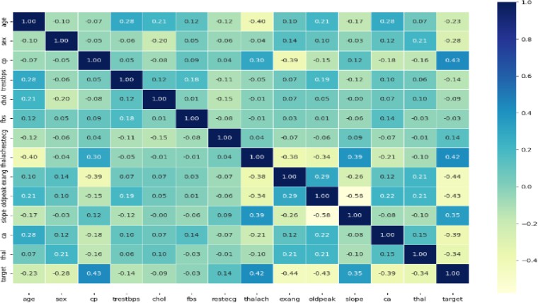
In order to prevent minor outliers from influencing the final diagnosis, only severe cases were eliminated. These were identified using equations (1) and (2), where the In- terquartile Range (IQR), a measure of data dispersion, along with Q1 and Q3 (lower and upper quartiles), were utilized. Instances exceeding (75% × Q3) + 3 × IQR (equation 1) or falling below (25% × Q1) 3 × IQR (equation 2) were excluded. Consequently, two instances out of the initial 303 were removed. A matrix of correlation coefficients was then created to evaluate the relationship between different features and outcomes. Figure 1 depicts the correlation matrix, with coefficients indicating both the strength and direction (positive or negative) of the associations between variables.

Figure 1

2) Verifying Disproportions

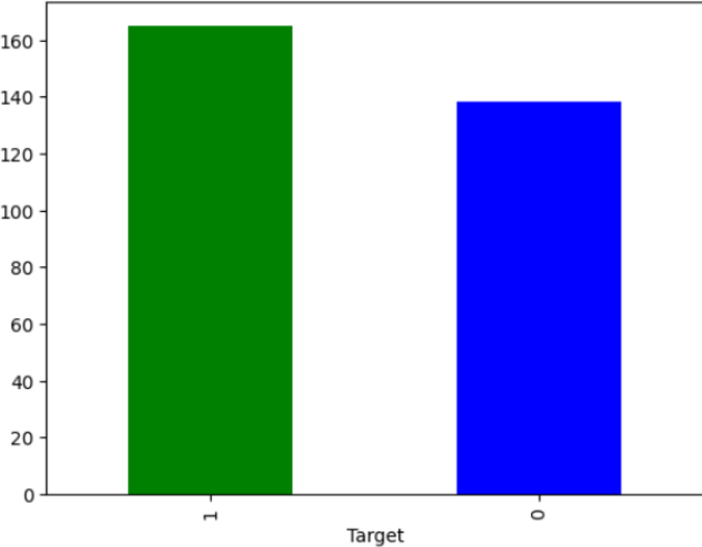
Prediction accuracy is impacted by output inconsistencies. In light of this, Figure 2 defines the ”objective” output balance. When checked, the data becomes equal between the two groups at a ratio of 9:11. Therefore, there is no need to make changes to the data.

Figure 2

3) Data Transformation

When multiple datasets are combined or the dataset con- tains data in disparate formats, transformation is applied. The nominal features in this instance were changed into factors such as here sex feature was in format male and female so we transformed it into 1 and 0 using nominal encoding technique.

4) Data Splitting

The testing set is used to test the model and forecast the result, while the training set is used to train the model. This is how data is typically divided in machine learning. This study employed hold-out, in which testing accounted for 20% of the data and training accounted for the remaining 80%.

C. Applied Algortihms

1. Random Forest Regression: A learning technique called random forest generates a lot of decision trees during training and delivers either the average estimate of each individual tree (regression) or the sample of the group (classification).
2. Naive Bayes (NB): Given a class, the features are assumed to be independent, making it ”naive” yet it has demonstrated effectiveness in various applications, such as text classification and spam filtering.
3. Support Vector Machine: SVM’s primary objective is to define a decisive boundary between distinct classes for accurate labeling predictions using one or more feature vectors.
4. Decision Tree: A machine learning technique called the decision tree algo- rithm makes predictions by using decision trees. The decisions and their outcomes are arranged in a tree-like structure.
5. Logistic Regression: Using binary distribution functions, A supervised machine learning method for estimating the likelihood of an observa- tion, event, or result is called logistic regression.
6. XGBoost: By merging predictions from weak and basic models, the supervised learning process known as gradient boosting aims to reliably forecast target variables.
7. KNN: It is employed to split tasks between two teams. KNN forms an information group whenever new information becomes available.

System Architecture

D. Evaluation Metrics

The machine learning model’s effectiveness and quality are assessed using evaluation measures. The best model in this research was selected using the assessment measures listed below:

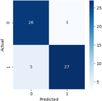
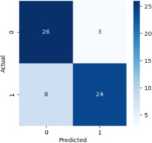
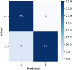
1) Confusion Matrix

The number of anticipated classes, N, is represented by the N*N matrix. As in this case, the confusion matrix has dimensions of 2*2 for a prediction issue with two alternative outcomes.

The proper and wrong prediction counts, broken down by class, make up the matrix’s components. A True Positive, for instance, is the quantity of the correctly categorized Positive class (heart disease cases, in this example). Comparably, the quantity of accurately identified Negative classes—in this example, the quantity of properly projected absences of heart disease—denotes a True Negative.

2) Accuracy

The % age of all forecasts that were correctly classified, as indicated by the confusion matrix and calculated using the subsequent equation:

Accuracy =             TP + TN            

                   TP + TN + FP + FN

3) Precision

The following equation may be used to get the proportion of positively categorized instances that were correctly classified from the confusion matrix:

Precision =   TP       

                  TP + FP

4) Recall

The percentage of real positive results that were properly recognized from the confusion matrix may be obtained using the following equation:

Precision =         TP     

                    TP + FN

5) F1-Score

If the objective is to obtain the highest accuracy and recall, the F measure—which is obtained from the confusion matrix using the following equation—would be the best choice since it provides the harmonic average of both the recall and the precision values in classification problems:

          2 · precision · recall

F 1 = precision + recall                                  (4)

III. RESULT AND ANALYSIS

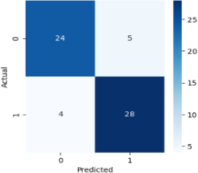
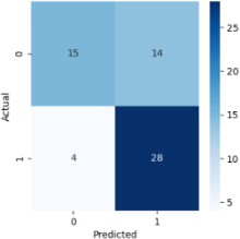
Seven algorithms based on machine learning were selected to create a heart disease prediction model, and the best final model was then derived from the outcomes of three distinct stages. Using every feature in the data, a prediction is created in the first stage. Using the chosen characteristics, a forecast is created in the second stage. Afterwards, hyperparameter adjustment is used in the final prediction step to enhance performance, and the more effective model is then used to produce the optimal model. Based on the accuracy displayed in Figure 5 and the confusion matrix, Table III presents the outcomes for every model utilizing all of the characteristics.

A. Confusion Matrix

1) Logistic Regression

2) Random Forest

3) Support Vector Classifier

4) Naive Bayes

5) Decision Tree

6) XGBoost

7) KNN

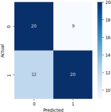
Now from above analysis we came to know that logistic regression and random forest regression both models fits well on the dataset with 89% and 85% accuracy respectively.So now in second stage we will try to find out features from this to models that are really important in the model creation and trying to remove the features that are less important. After applying feature selection technique on the Logistic Regression model we came to know cp, restecg, thalach, exang, oldpeak, slope, thal are the important features as shown in the figure below.

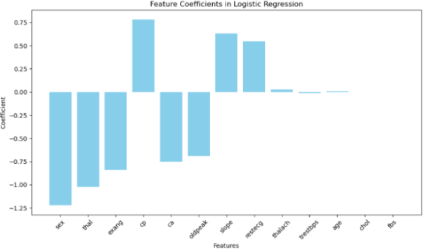
So we removed all the other features and created a model again

But according to our analysis this model has underperformed with respect to this first model we created as it shows only 75% accuracy. After that we applied feature selection techniques on random Forest regressor models. We discovered that, as indicated in the figure below, the following traits are significant: cp, trestbps, chol, thalach, exang, oldpeak, slope, ca, and thal.

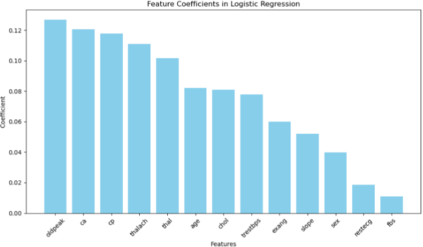
So now after keeping the desired features we created a model again.But here also the model under performed with the accuracy of 78%.

Now in the Third stage then we tried to perform hyperpa- rameter tuning on the logistic regression and random forest both models. First for Logistic regression we took all this parameters,

’C’: [0.001, 0.01, 0.1, 1, 10, 100],

‘penalty’: [’l1’, ’l2’],

’solver’: [’liblinear’, ’newton-cg’, ’lbfgs’, ’sag’, ’saga’]

Now using GridSearchCV we find out best parameters the logistic regression model and those where

After creating a model using this hyperparameter it gives accuracy of 85%.

Similarly for Random Forest Regressor we took this param- eters,

’nestimators′ : [100, 200, 300], ’maxdepth′ : [None, 10, 20, 30], ’minsamplessplit′ : [2, 5, 10],

’minsamplesleaf′ : [1, 2, 4],

’maxf eatures′ : [′auto′,′ sqrt′,′ log2′]

Again we used GridSearchCV and found out the best fit hyperparameters those are

Best Hyperparameters : ‘max depth’: None,’max fea- tures’:auto, ‘min samples leaf’:2, min samples split’:10, ‘n estimators’: 300

After creating a model using this hyperparameter it gives accuracy of 80%.

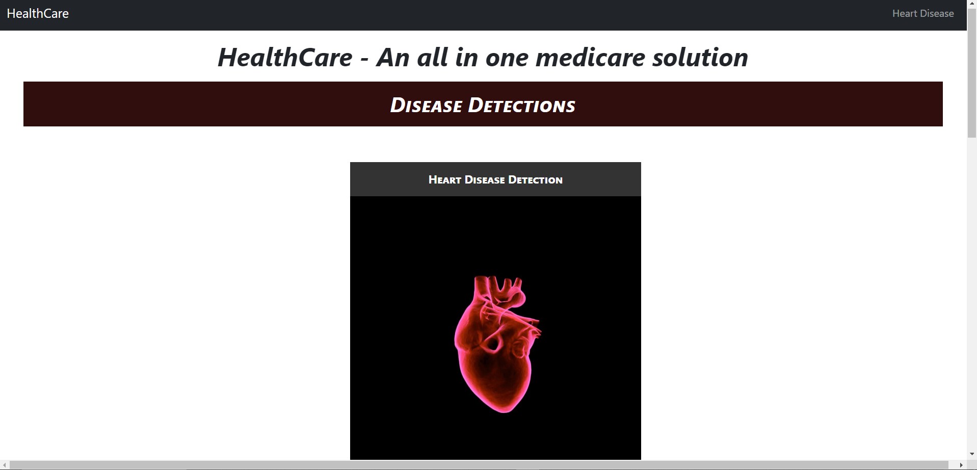
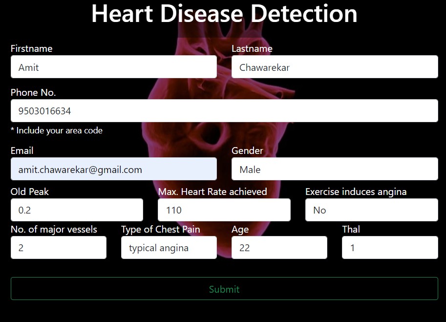
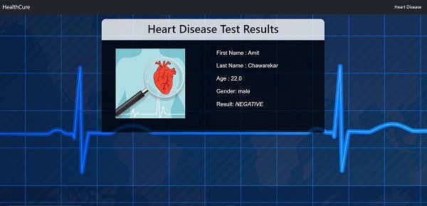
Our System is deployed using python flask server.

Homepage

Prediction Form

Report

Conclusion

In summary, machine learning’s application in predicting heart disease is a significant breakthrough in healthcare. By combining advanced algorithms with extensive datasets, these tools show promise in early detection and risk assessment. The capacity to recognize subtle patterns in diverse patient data allows for more accurate predictions, leading to timely interventions and better outcomes. However, ongoing refine- ment and validation with real-world clinical data are crucial for reliability and applicability across diverse populations. As technology advances, collaboration between healthcare professionals, data scientists, and policymakers is vital to fully leverage machine learning in alleviating the global burden of heart disease.

References

[1] C. Boukhatem, H. Y. Youssef and A. B. Nassif, ”Heart Disease Pre- diction Using Machine Learning,” 2022 Advances in Science and En- gineering Technology International Conferences (ASET), Dubai, United Arab Emirates, 2022, pp. 1-6, doi: 10.1109/ASET53988.2022.9734880. [2] S. Mohan, C. Thirumalai and G. Srivastava, ”Effective Heart Dis- ease Prediction Using Hybrid Machine Learning Techniques,” in IEEE Access, vol. 7, pp. 81542-81554, 2019, doi: 10.1109/AC- CESS.2019.2923707. [3] V. Sharma, S. Yadav and M. Gupta, ”Heart Disease Prediction us- ing Machine Learning Techniques,” 2020 2nd International Confer- ence on Advances in Computing, Communication Control and Net- working (ICACCCN), Greater Noida, India, 2020, pp. 177-181, doi: 10.1109/ICACCCN51052.2020.9362842 [4] T. M. Ghazal, A. Ibrahim, A. S. Akram, Z. H. Qaisar, S. Munir and [5] S. Islam, ”Heart Disease Prediction Using Machine Learning,” 2023 International Conference on Business Analytics for Technology and Security (ICBATS), Dubai, United Arab Emirates, 2023, pp. 1-6, doi: 10.1109/ICBATS57792.2023.10111368. [6] Akhtar, Nayab. (2021). Heart Disease Prediction. [7] K. Joshi, G. A. Reddy, S. Kumar, H. Anandaram, A. Gupta and [8] H. Gupta, ”Analysis of Heart Disease Prediction using Various Ma- chine Learning Techniques: A Review Study,” 2023 International Conference on Device Intelligence, Computing and Communication Technologies, (DICCT), Dehradun, India, 2023, pp. 105-109, doi: 10.1109/DICCT56244.2023.10110139. [9] S. Sivakumar and T. C. Pramod, ”Comprehensive Analysis of Heart Dis- ease Prediction: Machine Learning Approach,” 2022 IEEE 3rd Global Conference for Advancement in Technology (GCAT), Bangalore, India, 2022, pp. 1-7, doi: 10.1109/GCAT55367.2022.9972035. [10] S. Ibrahim, N. Salhab and A. E. Falou, ”Heart disease Prediction using Machine Learning,” 2023 1st International Conference on Advanced Innovations in Smart Cities (ICAISC), Jeddah, Saudi Arabia, 2023, pp. 1-6, doi: 10.1109/ICAISC56366.2023.10085522. [11] P. Ramprakash, R. Sarumathi, R. Mowriya and S. Nithyavish- nupriya, ”Heart Disease Prediction Using Deep Neural Network,” 2020 International Conference on Inventive Computation Tech- nologies (ICICT), Coimbatore, India, 2020, pp. 666-670, doi: 10.1109/ICICT48043.2020.9112443. [12] A. Gavhane, G. Kokkula, I. Pandya and K. Devadkar, ”Prediction of Heart Disease Using Machine Learning,” 2018 Second Inter- national Conference on Electronics, Communication and Aerospace Technology (ICECA), Coimbatore, India, 2018, pp. 1275-1278, doi: 10.1109/ICECA.2018.84749 [13] P. Divyasri, D. SreeLakshmi, P. Sathvika, P. Teja and T. V. Charan, ”Cardiovascular Disease Prediction Using Machine Learning,” 2023 6th International Conference on Information Systems and Computer Networks (ISCON), Mathura, India, 2023, pp. 1-6, doi: 10.1109/IS- CON57294.2023.10112052. [14] L. P. Koyi, T. Borra and G. L. V. Prasad, ”A Research Survey on State of the art Heart Disease Prediction Systems,” 2021 International Confer- ence on Artificial Intelligence and Smart Systems (ICAIS), Coimbatore, India, 2021, pp. 799-806, doi: 10.1109/ICAIS50930.2021.9395785. [15] A. H. Chen, S. Y. Huang, P. S. Hong, C. H. Cheng and E. J. Lin, ”HDPS: Heart disease prediction system,” 2011 Computing in Cardiol- ogy, Hangzhou, China, 2011, pp. 557-560. [16] M. Rasheed et al., ”Heart Disease Prediction Using Machine Learning Method,” 2022 International Conference on Cyber Re- silience (ICCR), Dubai, United Arab Emirates, 2022, pp. 1-6, doi: 10.1109/ICCR56254.2022.9995736. [17] J. Thomas and R. T. Princy, ”Human heart disease prediction system using data mining techniques,” 2016 International Conference on Circuit, Power and Computing Technologies (ICCPCT), Nagercoil, 2016, pp. 1- 5, doi: 10.1109/ICCPCT.2016.7530265.

Copyright

Copyright © 2024 Amit Chawarekar, Siddhant Divekar, Prof. Pallavi Thakur . This is an open access article distributed under the Creative Commons Attribution License, which permits unrestricted use, distribution, and reproduction in any medium, provided the original work is properly cited.