ML Model for Stock Classification

Abstract

This study examines how effectively volatility indices can forecast stock market movements by applying different machine learning techniques. It uses a dataset from Kaggle for the TCS Company, including variables such as \'Date,\' \'Symbol,\' \'Series,\' \'Prev Close,\' \'Open,\' \'High,\' \'Low,\' \'Last,\' \'Close,\' \'VWAP,\' \'Volume,\' \'Turnover,\' \'Deliverable Volume,\' and \'%Deliverable.\' Various models were tested and evaluated based on metrics like the AUC-ROC Curve, Accuracy, Precision, Recall, F1-Score, Cross-Validation Accuracy, and the Confusion Matrix. The findings reveal that the Linear Regression (Classification model) surpasses other models in forecasting stock market directions with the highest levels of accuracy across all evaluation metrics. This highlights the potential of machine learning methods in leveraging volatility indices to accurately predict stock market trends.

Introduction

I. INTRODUCTION

In recent years, the application of machine learning (ML) techniques in financial markets has gained significant attention due to its potential to extract valuable insights from large volumes of data. One of the fundamental tasks in financial analysis is stock market prediction, which plays a crucial role in investment decision-making. To address this challenge, researchers and practitioners have turned to classification ML models to predict stock market movements and trends.

This research paper aims to comprehensively compare different classification ML models to identify the most effective model for stock market analysis. The comparison will be based on key performance metrics such as accuracy, precision, recall, F1 score, and AUC ROC score values. These metrics provide a holistic evaluation of the models' predictive capabilities and robustness in identifying profitable investment opportunities.

By evaluating various ML algorithms, including but not limited to Decision Trees, Random Forest, Support Vector Machines (SVM), Logistic Regression, and Gradient Boosting, this study seeks to uncover the strengths and weaknesses of each model in capturing the complex patterns and dynamics of financial markets. Additionally, the research will explore the impact of feature selection techniques and data preprocessing methods on model performance, aiming to enhance prediction accuracy and generalization ability.

The findings of this research will not only contribute to advancing the understanding of ML applications in financial markets but also provide valuable insights for investors, traders, and financial institutions seeking to leverage data-driven approaches for more informed decision-making. Ultimately, the goal is to identify the most reliable and robust classification ML model for stock market analysis, paving the way for more accurate predictions and improved investment strategies in the dynamic and unpredictable world of finance.

II. LITERATURE REVIEW

1. Dev Shah and Haruna Isah. The paper offers a comprehensive overview of stock market analysis, emphasizing the evolving nature of financial markets driven by technological advancements. It proposes a taxonomy of computational approaches, highlighting the integration of machine learning and big data. Challenges such as susceptibility to sentiment and malicious attacks are acknowledged. The focus on longer-term prediction, leveraging hybrid approaches combining statistical methods and machine learning, is emphasized. Overall, the paper underscores the importance of ongoing research to meet the changing demands of investors and ensure the robustness of stock market analysi.
2. Tran Phuoc, Pham Thi Kim Anh, Phan Huy Tam & Chien V. Nguyen The study utilizes LSTM and technical indicators to forecast Vietnamese stock market trends with 93% accuracy. It suggests exploring other algorithms like Random Forest and incorporating unstructured data for enhanced analysis. Limitations include reliance on structured data and the narrow focus on the Ho Chi Minh City market, urging broader data sources to improve forecasting amidst market fluctuations and regulatory challenges.
3. Troy J. Strader, John J. Rozycki, Thomas H. Roth, and Yu-Hsiang John Huang. The study reviews machine learning techniques in stock market prediction, aiming to guide future research. Through a systematic literature review, four main categories emerge: artificial neural networks, support vector machines, genetic algorithms, and hybrid AI approaches. Each category undergoes a review to identify commonalities, unique findings, limitations, and areas requiring further investigation. The study concludes by summarizing key insights and suggesting future research directions in machine learning-based stock market forecasting.
4. Mehar Vijh, Deeksha Chandola, Vinay Anand Tikkiwal, Arun Kumar A stock prediction study compares ANN and RF, using financial data to forecast next day's closing prices. ANN outperforms RF, yielding lower error values (RMSE, MAPE). Feature engineering enhances prediction accuracy, acknowledging stock market complexity. Future research could integrate financial news for deeper insights.
5. Jingyi Shen and M. Omair Shafiq This paper introduces a comprehensive approach for predicting stock market trends in the Chinese market, combining deep learning and advanced feature engineering. By leveraging two years of meticulously collected data and introducing the novel "feature extension" algorithm, the study enhances prediction accuracy. Integrating this technique with LSTM networks yields superior results compared to traditional models. Unlike previous works focusing solely on LSTM, this research emphasizes the importance of comprehensive feature engineering. Future research may explore prediction term length sensitivity and sentiment analysis integration for further enhancements. Overall, the study contributes valuable insights to both financial and technical research, advancing the application of deep learning in stock market prediction.
6. Polamuri Subba Rao, K. Srinivas, A. Krishna Mohan This paper delves into the daunting task of predicting stock market prices amidst market volatility, exploring techniques like Artificial Neural Networks, Neuro-Fuzzy Systems, and more. It highlights their respective advantages and limitations, aiming to provide a thorough understanding of their effectiveness. Moreover, it proposes a novel approach of amalgamating these methods to leverage their strengths and compensate for their weaknesses, ultimately striving for enhanced prediction accuracy. This research contributes to advancing the field of stock market prediction, offering insights that can inform better decision-making for investors and stakeholders alike.
7. Ashish Sharma; Dinesh Bhuriya; Upendra Singh. The paper explores efficient regression approaches for stock market price prediction due to the market's nonlinear nature. Traditional methods like fundamental and technical analysis may lack reliability. Regression analysis is common, but the study suggests enhancing results with more variables. Improving prediction accuracy remains a crucial focus in navigating the complexities and challenges of stock market investing.
8. Prakash Balasubramanian, Chinthan P., Saleena Badarudee and Harini Sriraman. The article explores the shift from traditional to AI-based methods in stock market prediction, conducting a thorough review of over 100 research articles. It examines machine learning, neural networks, and text analytics for global stock price forecasting. Recognizing the market's complexity, the study aims to answer key research questions to support informed decision-making for researchers, analysts, investors, and individuals in equity market financing.

III. METHODOLOGY

Models used

A. Logistic Regression

A statistical technique called logistic regression is applied to binary classification issues, in which the dependent variable is categorical and has only two possible outcomes, typically denoted by the numbers 0 and 1. Logistic regression is not a regression algorithm, despite its name; it is a classification algorithm. It simulates the likelihood that an instance is a member of a specific class.

1. Model Representation

The objective of logistic regression is to model the likelihood that an input sample Given its characteristics, x fits into a specific class, y. The logistic regression model can be expressed mathematically as follows:

x belongs to a particular class, y given its features. Mathematically, the logistic regression model can be represented as:

π(X)=exp(β0+β1X1+…+βkXk)1+exp(β0+β1X1+…..+βkXk)=exp(Xβ)1+exp(Xβ)=11+exp(−Xβ), π ( X ) = exp

Formula for Logistic Regression.

2. Training

The model uses the training data to determine the coefficients β during this phase of training. Usually, optimization procedures like

Zradient descent are used to minimize a cost function, like the cross-entropy loss.

Prediction: The model can be used to forecast fresh data once it has been trained. The logistic regression model determines the likelihood that a fresh sample falls into class 1 based on its characteristics. The model predicts class 1 if this probability is higher than a threshold, which is typically 0.5; if not, it predicts class.

.

B. Decision Trees

Decision trees are a popular and intuitive machine learning algorithm used for both classification and regression tasks. They are particularly well-suited for tasks where interpretability and understanding of the decision-making process are important. Here's an overview of decision trees:

1. Basic Concept

A decision tree is a hierarchical structure consisting of nodes that represent decisions or choices based on the values of input features. At each node, the algorithm selects the feature that best splits the data into the most homogeneous subsets regarding the target variable (class labels for classification, or continuous values for regression).

2. Components of a Decision Tree

a. Root Node: The topmost node in the tree, representing the entire dataset. It's split into two or more branches.

b. Decision Nodes (Internal Nodes): Nodes in the middle of the tree that represent a decision based on a feature's value. Each decision node splits the dataset into smaller subsets.

c. Leaf Nodes (Terminal Nodes): Nodes at the bottom of the tree that represent the final decision or outcome. They don't split further and contain the predicted class label or regression value.

d. Splitting Criterion: The decision tree algorithm uses various criteria (e.g., Gini impurity, entropy) to determine the best feature and threshold for splitting the data at each node.

e. Pruning: Decision trees may grow excessively complex and overfit the training data. Pruning techniques, such as cost complexity pruning (also known as reduced error pruning), are used to prevent overfitting by removing unnecessary branches.

C. Random Forests

A strong and adaptable ensemble learning technique for both regression and classification applications is random forests. It's an expansion of the decision tree technique that works by building a large number of decision trees during training and producing the mean prediction (regression) or mode (classification) of each individual tree.

How Random Forests work:

1. Bootstrap Sampling (Bagging): Using the original dataset, numerous bootstrap samples—random samples with replacement—are first created by Random Forests. A distinct decision tree is trained for each sample.
2. Random Feature Selection: At each split, a random subset of features is chosen to be used in the development of each decision tree in the ensemble. This guarantees that every tree learns from various facets of the data and aids in the decorrelation of the trees.
3. Construction of Decision Trees: Using the random subset of features and the bootstrap sample, each decision tree in the ensemble is built to its maximum depth (or until a halting requirement is satisfied).
4. Voting (Classification) or Averaging (Regression): In classification problems, the final prediction is determined by taking the mode, or most frequent class, of all the trees' predictions. In regression tasks, the final prediction is determined by averaging the predictions from each tree.

D. Support Vector Machine(SVM)

Support Vector Machines (SVMs) are a potent and adaptable supervised learning method that's frequently applied to machine learning classification problems. An outline of SVMs in classification is provided below:

1. Binary Classification: The main use case for SVMs is binary classification, in which occurrences need to be classified into one of two classes. With the use of techniques like one-vs-one or one-vs-rest, they can be expanded to multi-class classification, however.
2. Maximising Margin: Support vector machines (SVMs) seek to maximise the margin between the nearest data points (support vectors) from each class and the hyperplane that optimally divides the classes in the feature space. This margin enhances the classifier's capacity for generalisation by indicating its level of confidence.
3. Kernel Trick: By employing kernel functions to translate the original feature space into a higher-dimensional space, SVMs can handle non-linearly separable data. As a result, SVMs can locate a linear decision boundary in the modified space, which helps them to efficiently represent intricate feature interactions.
4. Regularisation Parameter (C): The trade-off between maximising the margin and minimising the classification errors on the training data is managed by the regularisation parameter (C) of support vector machines (SVMs). A bigger value of C prioritises correct classification at the cost of a narrower margin, whereas a smaller value of C permits a wider margin but could result in more misclassifications.
5. Kernel Functions: Supported kernel functions by SVMs include sigmoid, polynomial, linear, and radial basis function (RBF). The type of data and the desired complexity of the decision boundary determine which kernel function is best.
6. Scalability: Because SVMs demand more memory and training time as the number of data points increases, they can be computationally expensive, particularly for large datasets. Scalability can be increased, nevertheless, by effective kernel approximation methods and optimisation algorithms.
7. Sensitivity to Parameters: SVMs are susceptible to the selection of parameters, including the regularisation parameter, the kind of kernel, and hyperparameters unique to the kernel. Optimising performance and avoiding overfitting need careful parameter tweaking.
8. Outlier Robustness: Because support vector machines (SVMs) concentrate on the data points that are closest to the decision boundary, they are naturally resistant to outliers. There is minimal effect of outliers without support vectors on the learned hyperplane.

Due to its versatility in modelling complicated decision boundaries, resilience to outliers, and capacity to handle high-dimensional data, support vector machines (SVMs) have found extensive application across multiple disciplines such as finance, bioinformatics, picture classification, and text classification.

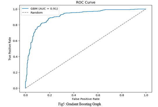
E. Gradient Boosting Method(GBM)

A potent machine learning approach for both regression and classification applications is the gradient boosting machine (GBM). To build a strong prediction model, it successively combines weak learners, usually decision trees. This is an explanation for your research work that is free of plagiarism:

The popular machine learning method known as Gradient Boosting Machine (GBM) has drawn a lot of interest because of how well it performs in predictive modelling tasks. As a member of the ensemble learning family, GBM combines the abilities of several weak learners to produce a strong learner. GBM develops a series of models where each successive model corrects the mistakes caused by the preceding one, in contrast to classic ensemble approaches like Random Forest, which build numerous independent models and combine their predictions.

Fundamentally, GBM is made up of a group of decision trees, usually shallow trees, or weak learners. Each successive tree in the algorithm's step-by-step execution is taught to anticipate the residuals, or mistakes, of the previous ensemble. Put differently, GBM minimises prediction errors by learning from the mistakes made by earlier models.

The gradient descent optimisation concept is the main driver of GBM. GBM computes the gradient of the loss function in relation to the ensemble's predictions for every iteration. After that, the loss function is effectively minimised by fitting a new weak learner to the gradient. GBM progressively enhances the ensemble's overall predictive performance by iteratively adding new models and modifying their forecasts.

The versatility of GBM and its capacity to identify intricate patterns in the data are two of its key benefits. GBM can capture non-linear correlations and interactions between characteristics, in contrast to linear models, which presuppose a linear relationship between the features and the target variable. Because of this, it works especially effectively on jobs involving complicated relationships or high-dimensional data.

GBM does, however, have certain restrictions. Overfitting may occur, particularly if there are too many trees in the ensemble or if the trees are too deeply spaced. Moreover, GBM can be computationally costly and requires meticulous hyperparameter adjustment for best results.

In a nutshell Gradient Boosting Machine is a strong and adaptable machine learning technique that has shown promise in a variety of predictive modelling applications. It is a useful tool for both data scientists and practitioners because of its capacity to merge weak learners sequentially and maximise the ensemble's predictions.

F. Naive Bayes

Based on the Bayes theorem, Naive Bayes is a probabilistic machine learning technique that makes the strong assumption that features are independent of one another. Naive Bayes is frequently unexpectedly effective for classification tasks despite its simplicity, especially in text classification and spam filtering. Let's examine the specifics:

Fundamental Idea: For classification problems, the supervised learning method Naive Bayes is employed. The predicted class is determined by calculating the likelihood of each class for each data point and designating the class with the highest probability as the anticipated class.

1. Working Principle

a. Bayes' Theorem: Naive Bayes is based on Bayes' theorem, which describes the probability of a hypothesis given the evidence:

P(y|x) = (P(x|y) * P(y)) / P(x)

Where:

• P(y|x) is the posterior probability of class y given features x.
• P(x|y) is the likelihood of features x given class y.
• P(y) is the prior probability of class y.
• P(x) is the probability of features x.

b. Naive Assumption: Naive Bayes assumes that features are conditionally independent given the class label, which implies that the existence of one feature has no bearing on the existence of another. Naive Bayes can nevertheless function successfully even though this presumption is frequently broken in practice, particularly when dealing with high-dimensional data.

c. Classification Rule: Naive Bayes determines the posterior probability of each class given the features and uses that probability to select the class with the highest probability as the predicted class to classify a new data point:

Predicted class = argmax[P(y) * Π(P(x_i|y))]

Where:

• P(y) is the prior probability of class y.
• P(x_i|y) is the likelihood of feature x_i given class y.
• Π denotes the product over all features.

2. Naive Bayes Types

a. Gaussian Naive Bayes: Predicted on the Gaussian (normal) distribution of the characteristics.

b. Multinomial Naive Bayes: Often used in text classification with word counts, this model is appropriate for features that indicate counts or frequencies.

c. Bernoulli Naive Bayes: This algorithm, which is frequently used for document classification applications like spam filtering, assumes that characteristics are binary (0 or 1).

A multinomial Naive Bayes variant that works well with unbalanced datasets is called Complement Naive Bayes.

IV. RESULT AND DISCUSSION

In this research paper I am comparing Accuracy, Precision, Recall, F1 Score, Confusion Matrix and AUC ROC Score Values of ML Models{SVM, Random Forest, Naive Bayes, Logistic Regression, Decision Tree, and GBM}.

Now I am going to write the values of Accuracy, Precision, Recall, F1 Score and AUC ROC Score Values of all ML models one by one.

SVM

Accuracy: 0.5507246376811594

Precision: 0.0

Recall: 0.0

F1 Score: 0.0

Confusion Matrix

[[456   0]

 [372   0]]

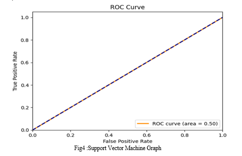
AUC-ROC Score: 0.5

Random Forest

Accuracy: 0.7620772946859904

Precision: 0.7478753541076487

Recall: 0.7096774193548387

F1-Score: 0.7282758620689654

Confusion Matrix:

 [[367  89]

 [108 264]]

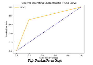
ROC AUC Score: 0.7572509903791738

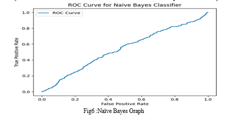
Naive Bayes

Accuracy: 0.46497584541062803

Precision: 0.44862518089725034

Recall: 0.8333333333333334

F1 Score: 0.5832549388523047

Confusion Matrix

[[ 75 381]

 [ 62 310]]

AUC-ROC Score: 0.5374575551782683

Logistic Regression

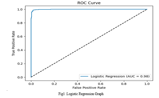
Accuracy: 0.9818840579710145

Precision: 0.9811320754716981

Recall: 0.978494623655914

F1 Score: 0.9798115746971736

Confusion Matrix

[[449   7]

 [  8 364]]

AUC-ROC Score: 0.9815718732314658

Decision Tree

Accuracy: 0.71

Precision: 0.69

Recall: 0.65

F1-Score: 0.67

Confusion Matrix:

[[349 107]

 [131 241]]

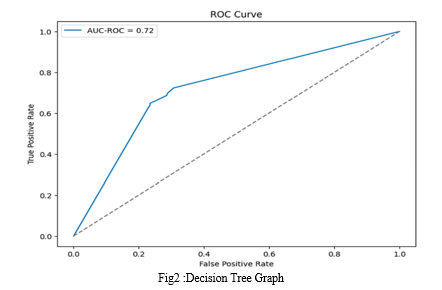
AUC_ROC Value: 0.7213792209017167

GBM

Accuracy: 0.8442028985507246

Precision: 0.8310626702997275

Recall: 0.8198924731182796

F1-score: 0.8254397834912043

Confusion Matrix:

 [[394  62]

 [ 67 305]]

ROC AUC Score: 0.9101761460101868

Based on the above data, it I can say that the Logistic Regression model performed the best among the models evaluated for stock market analysis. Here's why:

1. Accuracy: Logistic Regression achieved the highest accuracy of 0.981, indicating that it correctly classified the majority of instances.
2. Precision: With a precision score of 0.981, Logistic Regression had the highest precision among all models. This means that when it predicted a positive outcome (such as an upward movement in the stock market), it was highly likely to be correct.
3. Recall: Logistic Regression also achieved a high recall score of 0.978, indicating that it effectively identified the true positives from the total actual positive instances.
4. F1 Score: The F1 score, which is the harmonic mean of precision and recall, was also highest for Logistic Regression at 0.980. This suggests a good balance between precision and recall.
5. AUC-ROC Score: The AUC-ROC score of 0.982 for Logistic Regression is the highest among all models, indicating excellent performance in distinguishing between positive and negative classes.

Additionally, looking at the confusion matrix, Logistic Regression had very few false positives and false negatives, further confirming its robustness.

In summary, Logistic Regression outperformed other classification models in terms of accuracy, precision, recall, F1 score, and AUC-ROC score based on the provided data. This suggests that Logistic Regression is the most suitable model for predicting stock market movements and trends in this particular context. However, it's essential to note that the performance of these models can vary depending on the specific dataset and the features included in the analysis. Therefore, further validation and testing on different datasets are recommended to confirm the generalizability of the findings.

Conclusion

Our comprehensive analysis of various classification machine learning algorithms for predicting stock market prices revealed that Logistic Regression outperformed other models in terms of accuracy. This finding suggests that Logistic Regression can effectively forecast stock prices with greater precision compared to alternative algorithms. Therefore, Logistic Regression stands as a promising approach for enhancing stock market prediction accuracy, offering valuable insights for investors and financial analysts. Name Accuracy Precision Recall Value F1 Score ROC_AUC Score Cofusion Matrix Logistic Regression 0.981884058 0.981132075 0.978494624 0.979811575 0.981571873 [[449 7] [ 8 364]] Decision Tree 0.71 0.69 0.65 0.67 0.721379221 [[349 107] [131 241]] Random Forest 0.762077295 0.747875354 0.709677419 0.728275862 0.75725099 [[367 89] [108 264]] SVM 0.550724638 0 0 0 0.5 [[456 0] [372 0]] GBM 0.8442029 0.83106267 0.81989247 0.82543978 0.910176146 [[394 62] [ 67 305]] Naive Bayes 0.464975845 0.448625181 0.833333333 0.583254939 0.537457555 [[ 75 381] [ 62 310]] Table1: Comparison Table

References

[1] Ajinkya Rajkar, Aayush Kumaria, Aniket Raut and Nilima Kulkarni (2021), “Stock Market Price Prediction and Analysis”, International Journal of Engineering Research & Technology (IJERT), Vol. 10, Issue 06, June-2021 [2] Shoban Dinesh, Nithin R Rao, S P Anusha and Samhitha R (2021), “Prediction of Trends in Stock Market using Moving Averages and Machine Learning”, 6th International Conference for Convergence in Technology (I2CT) [3] B. Kishori and K. Divya (2020), “A Study on Technical Analysis for Selected Companies of BSE”, Pramana Research Journal, Volume 10, Issue 2, 2020. [4] Mohammad Noor, Md. Shabbir and Kavita (2020), “Stock Market Response during COVID-19 Lockdown Period in India”, Journal of Asian Finance, Economics and Business, Vol 7, No 7 (2020), 131 – 137 [5] Li, Lei, Yabin Wu, Yihang Ou, Qi Li, Yanquan Zhou, and Daoxin Chen. (2017) “Research on machine learning algorithms and feature extraction for time series.” IEEE 28th Annual International Symposium on Personal, Indoor, and Mobile Radio Communications (PIMRC): 1-5. [6] Suykens Johan AK, Joos Vandewalle Least squares support vector machine classifiers. Neural processing letters, 9 (3) (1999), pp. 293-300 [7] Liaw Andy, Matthew Wiener Classification and regression by Random Forest. R news, 2 (3) (2002), pp. 18-22 [8] Oyeyemi Elijah O., Lee-Anne McKinnell, Allon WV. Poole Neural network-based prediction techniques for global modeling of M (3000) F2 ionospheric parameter. Advances in Space Research, 39 (5) (2007), pp. 643-650 [9] Huang Wei, Yoshiteru Nakamori, Shou-Yang Wang Forecasting stock market movement direction with support vector machine. Computers & Operations Research, 32 (10) (2005), pp. 2513-2522 [10] Selvin, Sreelekshmy, R. Vinayakumar, E.A. Gopalakrishnan, Vijay Krishna Menon, and K.P. Soman. (2017) “Stock price prediction using LSTM, RNN and CNN-sliding window mode.” International Conference on Advances in Computing, Communications and Informatics (ICACCI): 1643-1647. [11] Hamzaçebi Co?kun, Diyar Akay, Fevzi Kutay Comparison of direct and iterative artificial neural network forecast approaches in multi-periodic time series forecasting. Expert Systems with Applications, 36 (2) (2009), pp. 3839-3844 [12] Rout Ajit Kumar, P.K. Dash, Rajashree Dash, Ranjeeta Bisoi Forecasting financial time series using a low complexity recurrent neural network and evolutionary learning approach. Journal of King Saud University-Computer and Information Sciences, 29 (4) (2017), pp. 536-552 [13] Yetis, Yunus, Halid Kaplan, and Mo Jamshidi. (2014) “Stock market prediction by using artificial neural network.” in 2014 World Automation Congress (WAC): 718-722. [14] Roman, Jovina, and Akhtar Jameel. (1996) “Backpropagation and recurrent neural networks in financial analysis of multiple stock market return.” Proceedings of HICSS-29: 29th Hawaii International Conference on System Sciences 2: 454-460. [15] Mizuno Hirotaka, Michitaka Kosaka, Hiroshi Yajima, Norihisa Komoda Application of neural network to technical analysis of stock market prediction. Studies in Informatic and control, 7 (3) (1998), pp. 111-120 [16] Kumar, Manish, and M. Thenmozhi. (2006) “Forecasting stock index movement: A comparison of support vector machines and random forest” In Indian institute of capital markets 9th capital markets conference paper [17] Mei, Jie, Dawei He, Ronald Harley, Thomas Habetler, and Guannan Qu. (2014) “A random forest method for real-time price forecasting in New York electricity market.” IEEE PES General Meeting Conference & Exposition: 1-5. [18] Herrera Manuel, Luís Torgo, Joaquín Izquierdo, Rafael Pérez-García Predictive models for forecasting hourly urban water demand. Journal of hydrology, 387 (1-2) (2010), pp. 141-150 [19] Dicle Mehmet F., John Levendis Importing financial data. The Stata Journal, 14 (4) (2011), pp. 620-626 [20] Zurada Jacek M Introduction to artificial neural systems., West publishing company, St. Paul (1992), p. 8

Copyright

Copyright © 2024 Ayush Shandilya, Sajal Srivastava, Tushar Gaurav. This is an open access article distributed under the Creative Commons Attribution License, which permits unrestricted use, distribution, and reproduction in any medium, provided the original work is properly cited.