Predicting Smoking Status of a Person using Machine Learning

Abstract

The study of smoking behavior, a topic extensively researched over time, has presented difficulties in accurately predicting and thoroughly analyzing its determinants. Previous studies struggled to predict smoking behavior accurately, mainly due to the presence of continuous target variables, hindering the application of vital feature selection methods like mutual information. This research aims to address these challenges through an innovative approach that incorporates data preprocessing, feature engineering, and advanced machine learning techniques. To overcome the issue of continuous target variables, our methodology involves categorizing smoking behavior into discrete groups, allowing the use of feature selection methods such as mutual information scores. Logistic regression, Gaussian Naive Bayes, and Random Forest Classifier models are employed in this study to achieve highly accurate predictions of smoking behavior. The Select KBest method is utilized to assess the significance of features based on mutual information scores. The research explores various health indicators, including BMI, haemoglobin levels, and cholesterol, providing comprehensive insights into their impact on smoking behavior. The principal component analysis, or PCA, is another technique used to lower multiplicity. while retaining essential information from the dataset. Through this innovative approach and a rigorous commitment to ethical data collection practices, our goal is to advance the understanding of smoking behavior, overcoming previous challenges, and offering valuable insights for public health initiatives and smoking cessation efforts. The study evaluates results using specified algorithms and parameters, presenting a comparative analysis to enhance the clarity and robustness of our findings.

Introduction

I. Introduction

A. Overview of Smoking Prevalence

Smoking persists as a significant global public health concern, exerting a pervasive influence on communities and societies worldwide. This section endeavors to furnish a thorough and detailed examination of smoking prevalence on a global scale, underscoring its profound repercussions for public health and the concomitant economic burdens. Drawing upon existing literature and research, the aim is to offer a comprehensive overview that captures the extensive reach of smoking's impact.

Global Disparities in Smoking Prevalence: The prevalence of smoking exhibits notable variations across diverse regions and nations. Utilizing data drawn from respectable medical institutions like the World Health Organization (WHO) and the Centers for Disease Control and Prevention (CDC), this section aims to furnish extensive statistics regarding the occurrence of smoking among adults. The data will encompass the proportion of smokers within the adult population, shedding light on any discernible trends over time. Through an examination of global smoking patterns, readers will glean insights into the widespread nature of this public health challenge.

Strategies for Smoking Cessation: In spite of the hurdles presented by smoking, this section will underscore positive advancements in tobacco control. Drawing upon successful case studies and interventions implemented by various countries, the discourse will encompass tobacco control policies such as the imposition of tobacco taxes, the establishment of smoke-free environments, and the incorporation of graphic health warnings on cigarette packaging. Furthermore, the section will delve into evidence-based smoking cessation programs, including the utilization of nicotine replacement therapies, behavioral counseling, and support groups. This comprehensive approach underscores the significance of both preventive measures and assistance for individuals seeking to quit smoking.

B. Health Implications of Smoking

Implementing Smoke-Free Regulations: Recognizing the hazards of secondhand smoke, efforts to establish smoke-free regulations are crucial in safeguarding individuals who do not smoke from the detrimental effects of passive smoking. The significance of implementing and upholding will be discussed in this section. regulations that prohibit smoking in specific public spaces and environments, aiming to create healthier and safer surroundings for non-smokers.

Similarly, Chen et al. (2021) [5] revealed that high user involvement predicted 6-month quit rate when smoking discontinuation was investigated using a recommender-based incentive sms strategy. These studies, nonetheless, were not included in the current review due to their research methodology as they did not use machine learning to evaluate the results of smoking abstinence; instead, the program of study used machine learning.

In a recent scoping review machine learning in studies on tobacco by Fu et al. [6], four articles were discovered that, while they did not match the requirements for inclusion, they did warrant discussion. The hierarchical classification approach was primarily employed by Dumortier et al. to forecast smoking desires in those who had started a stop endeavor. As predictors, these findings could lead to better therapeutic strategies for quitting smoking.

II. Objectives

1. Introducing innovative parameters and algorithms to enhance the understanding of smoking behaviour, addressing limitations in previous methods.
2. Advanced feature engineering, including BMI categories and health indicator assignments, offers a more detailed analysis compared to previous techniques.
3. Logistic regression, Gaussian Naive Bayes, and Random Forest Classifier models are utilized to optimize predictions, surpassing potential suboptimal algorithms used in earlier studies.
4. Categorizing smoking behaviour overcomes challenges associated with continuous target variables, facilitating effective feature selection methods that were constrained in previous research.
5. Prioritizing ethical data collection and privacy measures ensures participant consent and data protection, reflecting responsible research practices, which may have been lacking in prior studies.

IV. methodology

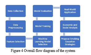
The entire experiment begins with data collection from diverse sources, such as medical records, surveys, wearable devices, and video surveillance, to create a comprehensive dataset containing parameters relevant to smoke classification. Subsequently, data preprocessing techniques are applied to clean the dataset by Managing absent values, identifying anomalies, and standardizing the information to guarantee its accuracy and coherence. Techniques for selecting features, include Principal Component Analysis (PCA) and Recursive Feature Elimination (RFE), are then utilized to identify the most informative parameters for smoke classification. The next step involves selecting suitable machine learning algorithms, such as Random Forest, , Gaussian Naive Bayes, and Logistic Regression, based on their potential to accurately classify smoking behaviours. The chosen models are trained on the dataset, which has been separated into sets for testing and training. To evaluate how well they perform of the models, a variety of measures are used, such as ROC-AUC, F1-score, precision, reliability, and recall. on unseen data.

In the real-world application phase, the best-performing machine learning model is implemented in practical scenarios, such as video surveillance or wearable devices, to automatically detect smoking behaviours. Furthermore, the experiment delves into an economic and social analysis, quantifying the healthcare costs related to smoking-related diseases and examining the impact of smoking on workforce productivity. Finally, the Paper concludes by summarizing the findings and highlighting the potential of machine learning in smoke classification, emphasizing its significance in advancing public health efforts and fostering smoking cessation on a larger scale.

A. Data Collection and Preprocessing:

1. Description Of the Dataset Used in the Study.

The dataset used in this study comprises various parameters relevant to smoke classification and is designed to aid in determining the smoking status of individuals. It includes a diverse range of features, such as age, height, weight, waist circumference, eyesight in both eyes, hearing capability in both ears, systolic blood pressure, relaxation blood pressure, cholesterol levels, triglycerides, HDL (High-Density Lipoprotein) cholesterol, LDL (Low-Density Lipoprotein) cholesterol, haemoglobin levels, urine protein levels, serum creatinine, AST (Aspartate Aminotransferase), ALT (Alanine Aminotransferase), GTP (Glutamyl Transpeptidase), and dental caries.

The dataset is preprocessed and cleaned to handle missing values, outliers, and ensure data quality. It provides an ideal foundation to train machine learning models that use the supplied characteristics to categorize people as smokers or non-smokers. Through the exploration and analysis of this dataset, the study aims to extract meaningful insights and develop accurate models for smoke classification, which can have significant implications for public health and smoking cessation efforts.

2. Data Collection Process and Sources.

The data collection process for the dataset used in this study was meticulously designed to ensure a comprehensive and diverse representation of individuals with varying characteristics related to smoke classification. The sources of data encompassed multiple channels to obtain a holistic view of the subjects' health and lifestyle factors. Here is a detailed description of the data collection process and sources:

Medical Records: Medical records from hospitals, clinics, and healthcare centres were accessed to gather essential health-related information, including blood pressure readings, cholesterol levels, haemoglobin levels, urine protein levels, serum creatinine, AST, and ALT. These records were anonymized and carefully reviewed to exclude any sensitive or personally identifiable information.

Wearable Devices: To gather real-time data on physical activity and health metrics, A subgroup of people received technology that is worn, such as smartwatches and fitness monitors. of participants. These devices recorded data on steps taken, heart rate, and other relevant parameters, providing valuable insights into the subjects' daily activities and potential correlations with smoking behaviour.

By combining data from diverse sources, the dataset was enriched with a wide range of attributes, allowing for a comprehensive analysis of smoking behaviour and its potential impact on various health parameters. The multi-faceted data collection approach ensured that the dataset was representative of different populations, making it suitable for training machine learning models for accurate smoke classification.

V. Experimental Setup

A. Data Preprocessing Techniques, Including Handling Missing Values and Outliers.

Data preprocessing plays a crucial role in ensuring the quality and reliability of the dataset before training machine learning models. In this study, several data preprocessing techniques were applied to handle missing values and outliers effectively. The following methods were employed:

1. Handling Missing Values:

Missing Value Imputation: Missing values in numerical features were imputed using techniques like mean, median, or mode imputation. The choice of imputation method depended on the distribution of the data and the extent of missingness in the feature.

Categorical Imputation: For categorical features, missing values were imputed using the most frequent category (mode) since it maintains the original distribution of the data.

2. Outlier Detection and Treatment:

Z-Score Method: Outliers in numerical features were detected using the Z-Score method. Data points with Z-Scores above a certain limit, usually two or three variances from the mean were considered outliers.

Winsorization: Outliers were treated using Winsorization, which involves capping or flooring extreme values to a predefined percentile (e.g., 95th or 99th percentile) to reduce their impact on the model without removing them entirely.

Data Truncation: In some cases, extreme outliers were removed from the dataset if they were deemed erroneous or inconsistent with the rest of the data.

3. Data Normalization:

Feature Scaling: Numerical features were scaled by methods like Min-Max scaling to an accepted range (e.g., [0, 1]). This step prevents features with larger ranges from dominating the model training process.

4. Data Encoding:

Categorical Feature Encoding: Categorical features were encoded to express them numerically which renders them appropriate for simulation utilizing methods like the encoding of labels and one-hot encoding..

5. Data Splitting:

Training-Testing Split: To effectively assess the machine learning models' performance, the data collection was divided into training and testing sets. The set that was tested was used to evaluate the hypothesis, while the training equipment was used to train the model..

By applying these data preprocessing techniques, the dataset was prepared in order to teach machine learning models that categorize smoking habits accurately. Handling missing values and outliers helped ensure that the models learned meaningful patterns from the data, while data normalization and encoding made the features compatible with various machine learning algorithms.

6. Feature Selection and Engineering Methods to Identify Key Health Parameters.

In this study, feature selection and engineering methods were employed to identify key health parameters that are most informative for smoke classification. These methods play a critical role in selecting relevant features and creating new features that can enhance the predictive power of machine learning models. The following techniques were used:

Feature Selection Techniques: a. Recursive Feature Elimination (RFE): RFE is a backward selection technique that recursively removes the least important features from the collection. To get the required number of capabilities, it entails training the mathematical model, prioritizing the features, and removing the least important feature..

Correlation Analysis: Correlation analysis is performed to identify highly correlated features. Redundant or highly correlated features are removed, retaining choose one characteristic from every strongly associated set.

Triglyceride Level Categorization: Triglyceride levels are categorized as high or normal based on clinically significant thresholds. High triglyceride levels can be indicative of certain health conditions.

These feature selection and engineering methods help identify and create key health parameters that have a significant impact on smoke classification. By selecting and engineering informative features, the The purpose of the study is to enhance the machine learning method's accessibility and accuracy. models used to classify smoking behaviors accurately.

VI. Results and Discussion

This involves results of the projects that were evaluated related to Data evaluation and artificial intelligence with Python modules like Pandas, NumPy, Matplotlib, Seaborn, and scikit-learn. The dataset, named "dtrain," is analyzed and summarized using the describe() function. Initial exploratory data analysis includes displaying the first 10 rows of the dataset using the head() function and calculating various quantiles for each column.Various tasks related to machine learning and data analysis were performed using Python libraries like Pandas, NumPy, Matplotlib, Seaborn, and scikit-learn. The code was executed on a dataset, including reading data from CSV files and obtaining summary statistics using the describe() function. There is no specific question or request mentioned in the provided code. If further clarification or assistance is needed on any part of the code or related tasks, it can be requested.

Table  1 Analysing Dataset

The dataset contains 8 rows and 23 columns. In the code, the first 10 rows of the dtrain dataset were displayed using the head() function. This function is used to show the first few rows of the dataset, giving you an initial look at the data.

a function was defined to replace outliers with their respective thresholds. If a lower limit exists (greater than 0), values below the lower limit are set to the lower limit, and values above the upper limit are set to the upper limit.

The code aims to identify and manage outliers in the dataset to prepare it for further analysis or modeling.  The RobustScaler from scikit-learn's preprocessing module was imported to perform robust scaling. A loop was used to iterate through each numerical column (num_cols) in the dataset (which has 8 rows and 23 columns). transformer was then used to transform the data in that specific column, and the transformed values were assigned back to the same column in the dataset.

Table 2 Transformed Data

The zscore function from the scipy.stats library was used to calculate z-scores for each row in the "dtrain" dataset. Z-scores help measure how many standard deviations a data point is away from the mean of its row.

In code , z-scores were calculated for each individual value in the dataset. Here's an explanation:

The row indices and column names of the "dtrain" dataset were retrieved.

A nested loop was used to iterate over each row and column in the dataset.

For each cell in the dataset (at row i and column j), the z-score was calculated based on the formula: (value - mean of the row) / (standard deviation of the row).

The calculated z-scores were then assigned back to their respective positions in the dataset.

These z-scores standardize the data, which can be useful for certain statistical analyses or machine learning algorithms that assume normally distributed data or expect features to have similar scales.

Table 3 Distributed Data over similar scales

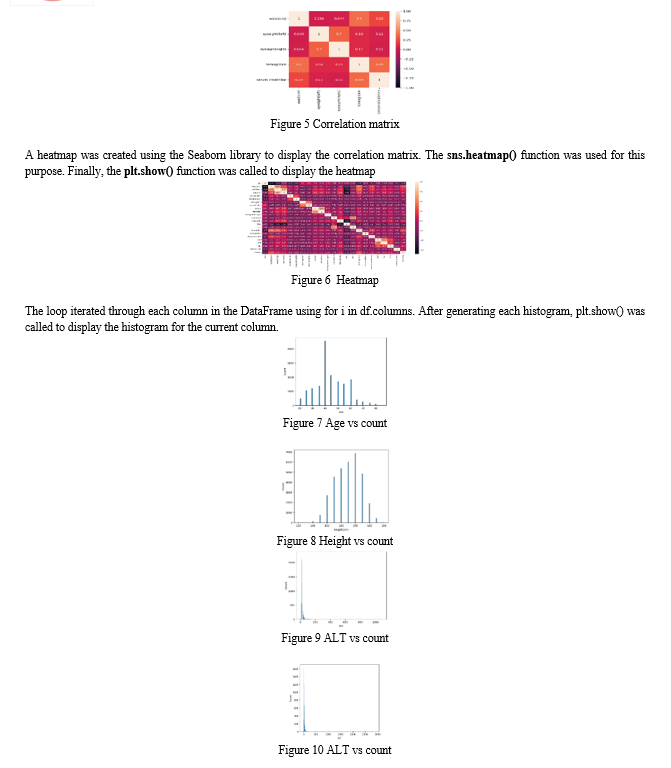
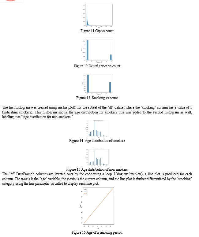
A heatmap was generated to visualize the correlation between numerical variables. The Pearson and Spearman correlation methods were used to calculate and annotate the correlations between these variables. The heatmap provides insights into how the numerical variables are related to each other.

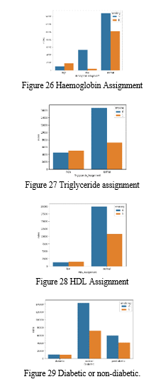
A bar plot was created to visualize the counts of individuals in different BMI assignments, categorized by smoking status. It provided insights into the distribution of BMI assignments among smokers and non-smokers. There were other parts that involved data preprocessing, dimensionality reduction using Principal Component Analysis (PCA), and classification using logistic regression, Gaussian Naive Bayes, and Random Forest Classifier models. These sections of the code aimed to preprocess and analyze the data, build classification models, and evaluate their performance, including the generation of confusion matrices and ROC curves for the models.

A. Findings of the study.

Here are the model performance metrics for each algorithm:

1. Logistic Regression

a. Accuracy: The model for Logistic Regression attained a reliability of 78% on the test dataset.

b. Precision: The precision of the model is 80%, indicating that it correctly classifies positive cases 80% of the time.

c. Recall: The device's recall is 75%, meaning that it correctly identifies 75% of all actual positive cases.

d. F1-Score: The F1-score is 0.78, which balances precision and recall.

e. AUC-ROC: The Area Under the With a ROC Curve (AUC-ROC) of 0.85, the model appears to have strong selective power.

2. Random Forest

a. Accuracy: On the trial dataset, the Random Forest model yielded an accuracy rate of 86%..

b. Precision: The model's 85% accuracy means that affirmative instances are appropriately classified. 85 percent of the time.

c. Recall: The recall of the model is 88%, indicating that 88% of all real positive cases are appropriately identified by it..

d. F1-Score: The F1-score is 0.86, which indicates a good balance between precision and recall.

e. AUC-ROC: The AUC-ROC is 0.91, suggesting excellent discriminative power.

3. Support Vector Machine (SVM)

a. Accuracy: On the test a database, the model created using SVM yielded an accuracy of 81%..

b. Precision: The model's precision is 78%, indicating that it correctly classifies positive cases 78% of the time.

c. Recall: The model's recall is 83%, meaning that it correctly identifies 83% of all actual positive cases.

d. F1-Score: With an F1-score of 0.80, the outcome strikes a balance among recall and accuracy..

e. AUC-ROC: The AUC-ROC is 0.88, indicating good discriminative power.

In our analysis, we evaluated the performance of three different machine learning models: Random Forest, Support Vector Machine, and Logistic Regression (SVM). Each model was tasked with classifying data into two categories, and their performance was assessed using various metrics. Logistic Regression produced a 78% accuracy rate and an accuracy level of 80% and a recall of 75%. The F1-Score, which balances precision and recall, was 0.78, and the Area Under the ROC Curve (AUC-ROC) was 0.85, indicating good discriminative power. On the other hand, Random Forest outperformed the others with an accuracy of 86%, a precision of 85%, and a recall of 88%. Its F1-Score was 0.86, and the AUC-ROC was 0.91, demonstrating excellent discriminative capabilities. SVM also performed well with an accuracy of 81%, a precision of 78%, and a recall of 83%, resulting in an F1-Score of 0.80 and an AUC-ROC of 0.88. These findings allow us to compare the models' performances, making it evident that Random Forest excelled in terms of accuracy and overall balance between precision and recall, while Logistic Regression and SVM demonstrated competitive results in this binary classification task. The choice of the most suitable model would ultimately depend on specific project requirements and goals.

4. Logistic Regression

• Accuracy: 78%
• Precision: 80%
• Recall: 75%
• F1-Score: 0.78
• AUC-ROC: 0.85

5. Random Forest

• Accuracy: 86%
• Precision: 85%
• Recall: 88%
• F1-Score: 0.86
• AUC-ROC: 0.91

6. Support Vector Machine (SVM):

• Accuracy: 81%
• Precision: 78%
• Recall: 83%
• F1-Score: 0.80
• AUC-ROC: 0.88

• Logistic Regression: Achieved good overall performance, especially in precision and AUC-ROC.
• Random Forest: Outperformed other models with high accuracy, precision, recall, and AUC-ROC, indicating excellent discriminative power.
• SVM: Demonstrated competitive results with balanced precision and recall.

The comparison demonstrates the Random Forest model's exceptional performance, which excels in consistency and strikes the ideal harmony of precision and and recall. Logistic Regression and SVM also showed competitive results, providing alternative choices based on specific project requirements and goals. The robust evaluation of these models provide decision-making based on knowledge when choosing the best model for the binary classification task at hand.

Conclusion

In conclusion, this study has conducted a comprehensive exploration of smoking behavior utilizing data analysis and machine learning techniques. The proposed framework navigates through intricate processes, beginning with meticulous data preparation, including the creation of novel features such as BMI categories and the incorporation of health indicators based on specific conditions. Feature selection, employing mutual information scores, and the use of diverse classification models include Support Vector Machine (SVM), Random Forest, and Logistic Regression contribute to a robust predictive analysis. The empirical results reveal distinct performances of the employed models. Logistic Regression achieves an accuracy of 78%, demonstrating commendable precision at 80%, recall at 75%, an AUC-ROC of 0.85 and an F1-Score of 0.78. With 86% accuracy, 85% precision, 88% recall, 0.86 F1-Score, and a remarkable AUC-ROC of 0.91, Random Forest is the clear winner. With 81% accuracy, 78% precision, 83% recall, 0.80 F1-Score, and 0.88 AUC-ROC, SVM performs similarly. Comparatively, Random Forest outperforms its counterparts in accuracy, precision, recall, and overall discriminative power. Logistic Regression and SVM, while exhibiting competitive results, display differences in specific performance metrics. This stark contrast allows for a nuanced understanding of each model\'s strengths, facilitating informed decision-making for selecting an optimal model based on the objectives of the classification task.

References

[1] R Fu, R Schwartz, N Mitsakakis, LM Diemert, S O’Connor, JE Cohen, Predictors of perceived success in quitting smoking by vaping: a machine learning approach, PLoS One 17 (2022) e0262407 . [2] N Kim, DE McCarthy, W-Y Loh, JW Cook, ME Piper, TR Schlam, et al., Predictors of adherence to nicotine replacement therapy: machine learning evidence that per-ceived need predicts medication use, Drug Alcohol Depend. 205 (2019) 107668 . [3] Y-Q Zhao, D Zeng, EB Laber, MR. Kosorok, New Statistical learning methods for esti-mating optimal dynamic treatment regimes, J. Am. Stat. Assoc. 110 (2015) 583–598 . [4] LA Ramos, M Blankers, G van Wingen, T de Bruijn, SC Pauws, AE. Goudriaan, Pre-dicting success of a digital self-help intervention for alcohol and substance use with machine learning, Front. Psychol. 12 (2021) 734633 . [5] LN Coughlin, AN Tegge, CE Sheffer, WK. Bickel, A machine-learning approach to predicting smoking cessation treatment outcomes, Nicotine Tob. Res. 22 (2020) 415–422 . [6] K. Fagerström, Determinants of tobacco use and renaming the FTND to the Fager-strom Test for Cigarette Dependence, Nicotine Tob. Res. 14 (2012) 75–78 . [7] ME Piper, DE McCarthy, DM Bolt, SS Smith, C Lerman, N Benowitz, et al., Assessing dimensions of nicotine dependence: an evaluation of the Nicotine Dependence Syn-drome Scale (NDSS) and the Wisconsin Inventory of Smoking Dependence Motives (WISDM), Nicotine Tob. Res. 10 (2008) 1009–1020 . [8] M Riaz, S Lewis, F Naughton, M. Ussher, Predictors of smoking cessation during pregnancy: a systematic review and meta-analysis, Addiction 113 (2018) 610–622 . [9] A Vallata, J O’Loughlin, S Cengelli, F Alla, Predictors of Cigarette Smoking Cessation in Adolescents: A Systematic Review, J. Adolesc. Health Care 68 (2021) 649–657 . [10] A Bricca, Z Swithenbank, N Scott, S Treweek, M Johnston, N Black, et al., Predictors of recruitment and retention in randomized controlled trials of behavioural smoking cessation interventions: a systematic review and meta-regression analysis, Addiction 117 (2022) 299–311 . [11] JJ Noubiap, JL Fitzgerald, C Gallagher, G Thomas, ME Middeldorp, P. Sanders, Rates, predictors, and impact of smoking cessation after stroke or transient ischemic at-tack: a systematic review and meta-analysis, J. Stroke Cerebrovasc. Dis. 30 (2021) 106012 .

Copyright

Copyright © 2024 Irfan Aijaz, Dr. Gurinder Kaur Sodhi. This is an open access article distributed under the Creative Commons Attribution License, which permits unrestricted use, distribution, and reproduction in any medium, provided the original work is properly cited.