Prediction of Abnormal Growth of Breast Cancer Cell Using Support Vector Machine

Abstract

Breast cancer is a serious health concern that affects millions of women worldwide. Early detection of breast cancer is crucial for effective treatment and improved survival rates. Artificial intelligence (AI) has shown great promise in the field of medical imaging and has been increasingly used for breast cancer detection. Cancer is one of the most dangerous diseases to humans, and yet no permanent cure has been developed for it. Breast cancer is one of the most common cancer types. According to the National Breast Cancer foundation, in 2020 alone, more than 276,000 new cases of invasive breast cancer and more than 48,000 non-invasive cases were diagnosed in the US. To put these figures in perspective, 64% of these cases are diagnosed early in the disease’s cycle, giving patients a 99% chance of survival. In this paper we develop a system for diagnosis, prognosis and prediction of breast cancer using AI. This will assist the doctors in diagnosis of the disease. In this research work, we systematically reviewed previous work done on detection and treatment of breast cancer using genetic sequencing or histopathological imaging with the help of deep learning and machine learning We use of AI for breast cancer detection, including studies that have used mammography, ultrasound, and magnetic resonance imaging (MRI) as imaging modalities. AI can also improve the accuracy and efficiency of breast cancer screening and diagnosis, as well as the challenges that must be addressed to ensure the successful integration of AI into clinical practice. However, further research and development are needed to optimize AI algorithms and ensure their safety and effectiveness in clinical practice. Breast cancer detection has emerged as a critical area of research, leveraging the power of Artificial Intelligence (AI) to enhance diagnostic accuracy and efficiency. Utilizing AI technologies, particularly deep learning, enables the development of robust and precise models for early breast cancer detection. These models analyze mammographic images, identifying subtle patterns indicative of malignancies that may escape human eye detection. Transfer learning, employing pre-trained neural network architectures, has demonstrated significant success in leveraging existing knowledge for improved performance. The integration of convolutional neural networks (CNNs) and image processing techniques empowers AI models to discern subtle abnormalities, aiding in the timely identification of potential breast tumors. Additionally, AI-driven diagnostic tools can streamline radiologists\' workflow, providing rapid and reliable assessments, ultimately contributing to early intervention and improved patient outcomes. As these technologies continue to evolve, the synergy between AI and breast cancer detection promises to revolutionize screening methods, fostering a paradigm shift towards more accurate, efficient, and accessible diagnostic practices in the realm of breast health.

Introduction

I. INTRODUCTION

Breast cancer is a prevalent and potentially life-threatening condition that affects a significant number of individuals worldwide. Early and accurate detection of breast cancer is pivotal for improving patient outcomes and facilitating timely intervention. In recent years, the application of machine learning (ML) techniques has garnered considerable attention in the field of medical diagnostics, offering promising avenues for enhancing the efficiency and accuracy of breast cancer detection.

The conventional methods for breast cancer diagnosis, such as mammography and biopsy, have proven efficacy, but they come with limitations, including potential discomfort, invasiveness, and subjectivity in interpretation. Machine learning, with its ability to analyze vast amounts of data and discern intricate patterns, has emerged as a valuable tool for complementing traditional diagnostic approaches.

This work aims to explore the application of machine learning in breast cancer detection, with a specific focus on Support Vector Machines (SVMs). SVMs are known for their robustness in handling complex classification tasks and have shown success in medical image analysis. By leveraging features extracted from breast cancer datasets, SVMs can contribute to creating predictive models that aid in distinguishing between malignant and benign tumors.

In this study, we delve into the details of how machine learning techniques, particularly SVMs, can be employed to analyze diverse features extracted from medical imaging data, clinical records, or genetic information. We will discuss the significance of data preprocessing, the choice of relevant features, and the fine-tuning of SVM parameters to optimize the model's performance.

Furthermore, the potential benefits of utilizing machine learning in breast cancer detection extend beyond improved accuracy. ML models can assist healthcare professionals in making more informed decisions, provide quantitative risk assessments, and contribute to the development of personalized treatment plans.

Through this exploration, we aim to shed light on the advancements in machine learning applications for breast cancer detection, emphasizing the potential transformative impact on early diagnosis, treatment planning, and overall patient care. The integration of machine learning into breast cancer detection holds great promise for ushering in a new era of precision medicine, where technological innovations enhance our ability to combat this significant health challenge.

II. LITERATURE REVIEW

1. "Breast Cancer Detection using Convolutional Neural Networks and Fuzzy Logic" by Ghahramani et al. (2020): This study proposes a breast cancer detection method using convolutional neural networks (CNNs) and fuzzy logic. The proposed method achieved an accuracy of 98.5% in breast cancer detection, which outperforms other state-of-the-art methods.
2. "Artificial Intelligence in Breast Cancer Screening and Diagnosis"by Alexander Muacevic and John R Adler (2022):Use Digital pathology and artificial intelligence. Computational radiology is used. Easy-to-access databases and user-friendly software.
3. "Breast Cancer Diagnosis using Artificial Neural Network Models" by R.R.Janghel , Anupam Shukla, Ritu Tiwari , Rahul Kala uses the Radial Basis Function Networks achive an accuracy of 95.82%.
4. Breast cancer detection using artificial intelligence techniques: A systematic literature review by Ali Bou Nassif*, Manar Abu Talib, Qassim Nasir, Yaman Afadar, Omar Elgendy (2022):Uses BPNN (Back propagation neural network). Produced 99.3% accuracy,
5. "A hybrid deep learning model for breast cancer diagnosis" by Zhou et al. (2021): This study proposes a hybrid deep learning model that combines convolutional neural networks (CNNs) and long short-term memory (LSTM) networks for breast cancer diagnosis. The proposed model achieved a high accuracy of 97.45%, which outperforms other state-of-the-art methods.
6. Breast Cancer Detection and classification Using Artificial Neural Networks.by Yousif A. Hamad , Konstantin Simonov Mohammad B. Naeem (2018) use Balance Contrast Enhancement Technique (BCET).
7. "Breast cancer detection using artificial intelligence: A review" by Albadr et al. (2021): This review article provides a comprehensive overview of the latest artificial intelligence techniques used for breast cancer detection. It includes discussions on the use of deep learning, machine learning, and other AI methods. The authors also highlight the challenges and future directions in this field.

III. METHODOLOGY

The methodology for breast cancer detection using artificial intelligence .

In the first part of our project we are goining to Predictive  breast cancer using machine learning . Breast Cancer occurs as a result of abnormal growth of cells in the breast tissue, commonly referred to as a Tumor. Since this build a model that can classify a breast cancer tumor using two training classification:

1 = Malignant (Cancerous) - Present

0 = Benign (Not Cancerous) -Absent

 We have collected the data form various sources. Main aim to find weather the cancer is malignant or can be predicted

1) DATA SOURCE:- The data set contains 569 samples of malignant and benign tumor cells.

 In 1st two columb we store unique id

Another 3-32 columb we store real-value features .

The first step is to visually inspect the new data set

We importing the data set .The simplest method is to retrieve the initial records by making a request through the Data Frame.

By this method we can cheak the no. Of cases as well as number of fields.

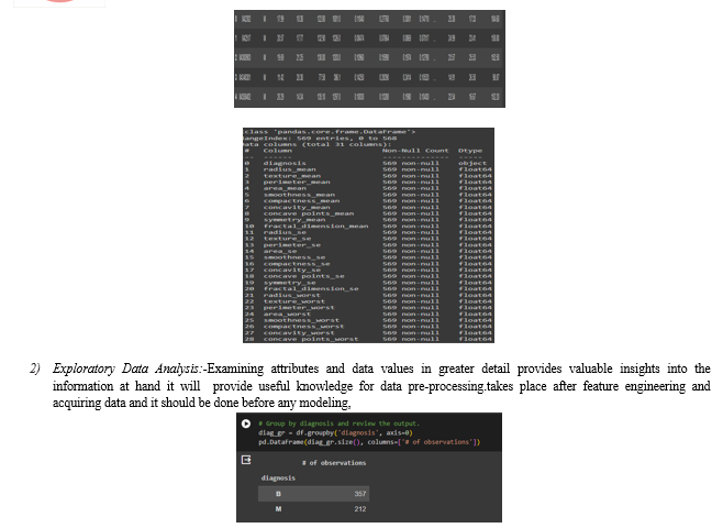
Here we show that the  grouping operation is a Data Frame that shows the count of observations for each unique value in the 'diagnosis' column. The result is displayed in a Data Frame with a single column named '# of observations', where the index represents the unique values in the 'diagnosis' column ('B' for benign and 'M' for malignant). It shows that there are 357 observations with a diagnosis of 'B' (benign) and 212 observations with a diagnosis of 'M' (malignant).

Next step is to explore the data. There are two approached used to examine the data using:

• Descriptive statistics:-a set of methods used to summarize and describe the main features of a data set, such as its central tendency, variability, and distribution.
• Visualization:-the graphical representation of information and data

Unimodal Data Visualizations

The primary objective of visualizing the data in this context is to identify which features are particularly influential in predicting malignant or benign cancer. Additionally, the visualization aims to uncover general trends that can guide us in the selection of models and hyper parameters.

• Histograms.:-

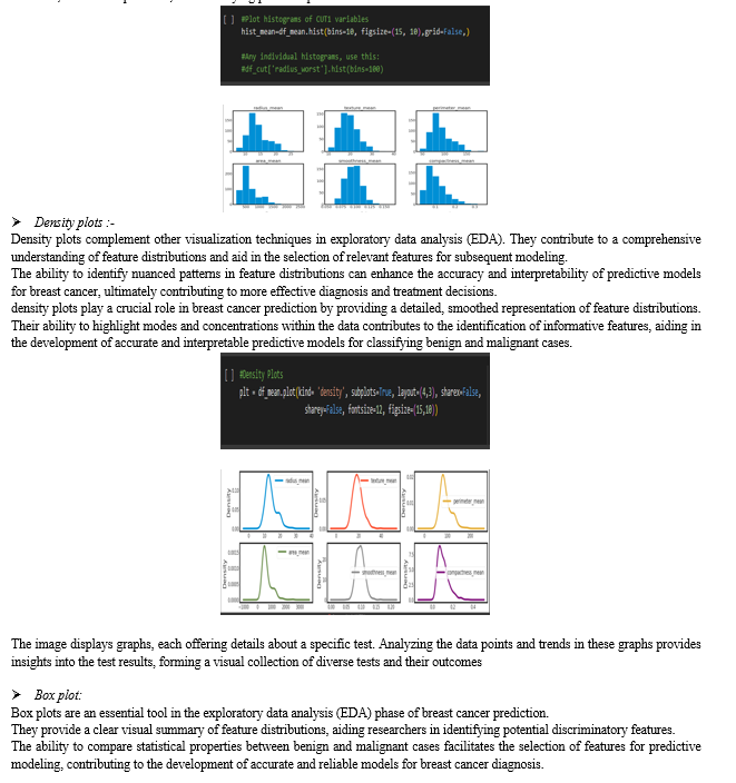
 A histogram is a graphical representation of the distribution of a data set. It provides a visual summary of the underlying frequency or probability distribution of a continuous variable. The process involves dividing the data into intervals, called bins, and counting the number of observations falling into each bin.

In Breast Cancer Prediction that show distinct patterns or significant differences in their histograms between benign and malignant cases may have predictive power and can be prioritized in subsequent modeling steps.

Its also to use Understanding the distribution, shape, spread, range, and variability of features within each class is crucial for feature selection, model interpretation, and identifying potential predictors.

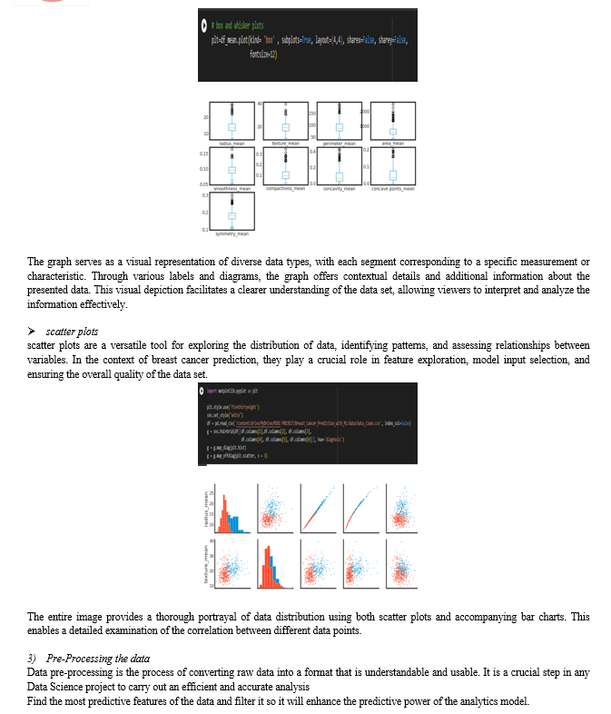
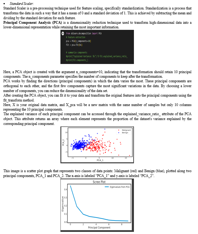
This is a Scree Plot, a graphical representation of the eigenvalues obtained from Principal Component Analysis (PCA). PCA is a statistical method used to reduce the dimensionality of data while retaining most of its variance. In this plot, the x-axis represents the principal components, which are ordered by their associated eigenvalues. The y-axis shows the eigenvalues, indicating the amount of variance each principal component explains. The plot displays a sharp decline in eigenvalue from the first to second principal component and then gradually approaches zero. This pattern helps in identifying the optimal number of principal components to retain for further analysi.

IV. PREDICTIVE MODEL USING SUPPORT VECTOR MACHINE (SVM)

The predictive model will be constructed using the Support Vector Machines (SVMs) learning algorithm. SVMs are widely recognized as a popular classification method, known for their effective approach to transforming nonlinear data. This transformation allows the application of a linear algorithm to fit a model to the data in an elegant manner.

SVMs offer the capability to create intricate decision boundaries, especially in scenarios with limited features. They perform effectively on datasets with both few and numerous features, but their scalability diminishes as the sample size increases.

While SVMs can handle datasets of up to 10,000 samples adequately, managing datasets exceeding 100,000 can pose challenges in terms of runtime and memory usage. Successful implementation of SVMs demands meticulous data preprocessing and parameter tuning. Consequently, many practitioners now favor tree-based models like random forests or gradient boosting, which often require minimal preprocessing.

Despite their strengths, SVM models present challenges in interpretability. Understanding the rationale behind a specific prediction can be challenging, making it difficult to explain the model to non-experts.

In kernel SVMs, crucial parameters include the regularization parameter (C), the selection of the kernel type (linear, radial basis function (RBF), or polynomial), and kernel-specific parameters. Both gamma and C play pivotal roles in controlling the model's complexity, where higher values contribute to increased complexity. Consequently, optimal configurations for these two parameters are often closely linked, emphasizing the need to adjust C and gamma concurrently for effective model tuning.

A. Classification with cross-validation

As discussed in data pre processing Splitting the data into training and test sets is crucial for preventing overfitting and promoting the generalization of the model to unseen data. Cross-validation takes this concept further by dividing the data into folds of similar sizes. During training, one fold serves as the holdout sample, and the model's performance is evaluated on this segment. The holdout sample is then reintegrated with the remaining folds, and a different fold becomes the new holdout sample. This process repeats until each fold has been utilized as a test or holdout sample. The cross-validation error, representing the expected performance of the classifier, is computed as the average of error rates observed on each holdout sample.

B. Model Accuracy: Receiver Operating Characteristic (ROC):-

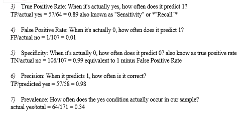
In statistical modeling and machine learning, the Area Under the Curve (AUC) is a frequently reported performance metric for model accuracy in binary classification problems. To comprehend the insights provided by the ROC curve, we can examine the confusion matrix. This matrix is a two-dimensional table where one axis represents the classifier model (vertical), and the other axis represents the ground truth (horizontal). Both of these axes can assume two values, as illustrated below.Either of these axes can take two values (as depicted).

 In an ROC curve, you plot “True Positive Rate” on the Y-axis and “False Positive Rate” on the X-axis, where the values “true positive”, “false negative”, “false positive”, and “true negative” are events (or their probabilities) as described above. The rates are defined according to the following:

• True positive rate (or sensitivity)}: tpr = tp / (tp + fn)
• False positive rate: fpr = fp / (fp + tn)
• True negative rate (or specificity): tnr = tn / (fp + tn)
• In all definitions, the denominator is a row margin in the above confusion matrix. Thus,one can express
• The true positive rate (tpr) as the probability that the model says "+" when the real value is indeed "+" (i.e., a conditional probability). However, this does not tell you how likely you are to be correct when calling "+" (i.e., the probability of a true positive, conditioned on the test result being "+")

V. OPTIMIZING THE SVM CLASSIFIER

Machine learning models are endowed with parameters that govern their behavior, and the tuning of these parameters is essential for optimizing their performance on specific problems. Since models often come with a multitude of parameters, identifying the most effective combination can be likened to a search problem. In the context of SVM (Support Vector Machine) Classification models using scikit-learn, the objective is to fine-tune the parameters to achieve the best predictive accuracy.

this part of the code demonstrates a systematic approach to finding the best hyperparameters for the SVM classifier through a grid search. This optimization process helps in improving the model's performance by fine-tuning the regularization parameter and kernel coefficient. The performance of the optimized model is then assessed using cross-validation. The choice of hyper parameters significantly impacts the SVM model's ability to generalize to new, unseen data.

the process of tuning two key parameters of the SVM algorithm (C and kernel) using Grid Search and Random Search in Python's scikit-learn library.

A. Tuning SVM Parameters:

C (Regularization Parameter): Controls the trade-off between a smooth decision boundary and classifying training points correctly. A smaller C encourages a larger-margin, simpler decision boundary, while a larger C penalizes training points that fall on the wrong side of the decision boundary.

Kernel: Specifies the type of hyperplane used for classification. Common choices include the Radial Basis Function (RBF) kernel, linear kernel, polynomial kernel, etc.

B. Default Parameters:

The default settings for SVM (SVC class in scikit-learn) use the RBF kernel with a C value set to 1.0. These defaults might not be optimal for all datasets, and tuning is required for better performance.

C. Grid Search Parameter Tuning:

Process:

Define a grid of hyperparameter values to explore. For example, different values for C and kernel.

Train the SVM model using each combination of hyperparameters.

Evaluate the model's performance using cross-validation (e.g., 10-fold cross-validation).

Identify the set of hyperparameters that yield the best performance.

D. Random Search Parameter Tuning:

Process:

Define distributions for each hyperparameter.

Randomly sample combinations of hyperparameters from these distributions.

Train the SVM model using each randomly sampled combination.

Evaluate the model's performance using cross-validation.

Identify the set of hyperparameters that yield the best performance.

Tuning these parameters is crucial for achieving the best possible SVM model for your specific dataset. Grid Search and Random Search are powerful tools for efficiently exploring the hyperparameter space and finding optimal combinations. The choice between them often depends on computational resources and the dimensionality of the hyperparameter space.

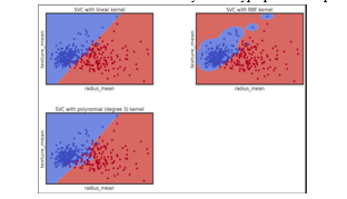
This image is a visual representation of how Support Vector Classification (SVC) with different kernels can be used to classify data points into two classes based on features “radius_mean” and “texture_mean”. The image consists of four scatter plots arranged in a 2x2 grid. Each plot represents a classification model using SVC with different kernel methods. The x-axis is labeled “radius_mean” and the y-axis is labeled “texture_mean” in all four plots. Blue and red dots represent two distinct classes or groups within the data. In the top-left plot, SVC with linear kernel is used. A straight line separates the blue and red dots indicating a linear boundary between classes. In the top-right plot, SVC with RBF kernel is used. An irregular boundary separates the groups, fitting closely around clusters of blue dots to distinguish them from red ones. In the bottom-left plot, SVC with polynomial (degree 3) kernel is used. A curved line separates blue from red dots indicating a polynomial boundary between classes. The OCR text at the bottom of the image lists the kernel method used for each plot along with the feature names.

Support Vector Machines often exhibit improved performance when the dataset is standardized. Standardization involves transforming the data such that all attributes have a mean value of zero and a standard deviation of one. This ensures that all features are on a comparable scale, preventing certain features from dominating others due to differences in their scales.

1. Dataset Overview: The dataset is divided into training and validation sets. The training set is used to train the SVM model, while the validation set is reserved for evaluating its performance on unseen data.
2. Standardization: Standardization is applied to the entire training dataset. This involves calculating the mean and standard deviation for each attribute in the training set. The mean value is subtracted from each attribute, and the result is divided by the standard deviation. This process centers the data around zero and scales it to have a standard deviation of one.
3. Applying the Same Transform to Validation Data: To ensure consistency, the same transformation (subtracting mean and dividing by standard deviation) applied to the training set is also performed on the input attributes of the validation dataset. This ensures that the validation data is on the same scale as the training data, allowing for fair and meaningful evaluation of the model's performance.

Standardizing the dataset is a crucial preprocessing step when utilizing Support Vector Machines for classification tasks. It contributes to the stability and effectiveness of the SVM model by placing all features on a standardized scale, thereby improving its ability to learn and generalize from the data.

VI. AUTOMATE THE ML PROCESS USING PIPELINES

Machine learning projects often follow standardized workflows, and in Python's scikit-learn library, Pipelines play a pivotal role in automating these processes.

By utilizing Pipelines, we can effectively address prevalent issues such as data leakage in the test harness, providing a streamlined and organized approach to machine learning workflows.

Python's scikit-learn offers a versatile Pipeline utility designed to automate various stages of the machine learning process.

Pipelines facilitate a systematic sequence of data transformations, allowing for a seamless chaining of operations that culminate in a modeling process. This structured approach enhances efficiency and clarity, making it easier to evaluate the performance of the entire workflow.

This work demonstrates the modelling of breast cancer as classification task using Support Vector Machine

The SVM performs better when the dataset is standardized so that all attributes have a mean value of zero and a standard deviation of one. We can calculate this from the entire training dataset and apply the same transform to the input attributes from the validation dataset.

This is a boxplot graph that compares the performance of different machine learning algorithms. The y-axis represents some form of measurement metric, and the x-axis has labels for each algorithm being compared: LR, LDA, KNN, CART, NB, and SVM . generates a boxplot for algorithm comparison using the matplotlib library. Below the code snippet is a boxplot titled “Algorithm Comparison.” The y-axis of the plot ranges from 0.825 to 1.000. Six different machine learning algorithms (LR, LDA, KNN, CART, NB, SVM) are compared on the x-axis. Each algorithm has its own box in the plot representing data distribution with outliers marked as individual points above or below the boxes 1.

Boxplots are a type of chart that is used to visualize how a given data (variable) is distributed using quartiles. It shows the minimum, maximum, median, first quartile and third quartile in the data set. Box plot is method to graphically show the spread of a numerical variable through quartiles

For a standard k-NN implementation, two key hyperparameters demand tuning:

The number of neighbors (k).

The choice of distance metric or similarity function.

These hyperparameters significantly impact the accuracy of the k-NN classifier. Utilizing a Grid object, we are prepared to execute a 10-fold cross-validation on a KNN model, using classification accuracy as the evaluation metric. Moreover, a parameter grid is established to iterate the 10-fold cross-validation process 30 times. In each iteration, the n_neighbors parameter assumes a different value from a specified list. It's important to note that we cannot simply provide GridSearchCV with a list; instead, we need to specify that n_neighbors should take on values from 1 through 30. To expedite computations, you can set n_jobs = -1 to enable parallel processing, provided it is supported by your computer and operating system.

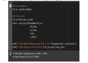
Final model traing accuracy

Final Model Training Accuracy: 0.940 +/- 0.034

? Final Accuracy on Test set: 0.94737

We have completed our prediction process  .

Now we start our detection process my using AI.

A. Data collection and processing:-

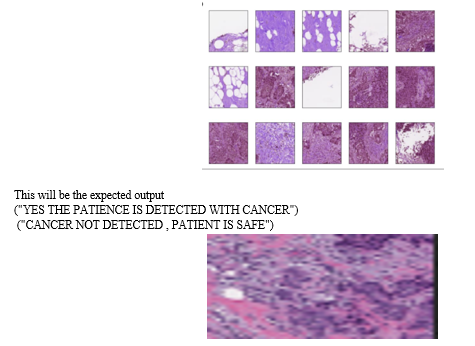
1. Dataset Description: The research utilizes a dataset containing breast cancer images, with each image categorized into two classes: 'No' (indicating absence of breast cancer) and 'Yes' (indicating the presence of breast cancer). This binary classification aligns with the nature of the diagnostic task.
2. Organization into DataFrame: To streamline data management and analysis, the image file paths and their corresponding labels are organized into a structured DataFrame. In Python, the Pandas library is employed for creating this DataFrame. Each row of the DataFrame represents an image instance, with columns containing information such as the file path and label. This organization facilitates efficient handling, indexing, and manipulation of the dataset during subsequent stages.

B. Visual Exploration:

A crucial step in understanding the dataset is the visual exploration of randomly selected images. This process involves randomly sampling images from the DataFrame and displaying them for visual inspection. Matplotlib, a popular plotting library in Python, is commonly used for this purpose. The goal is to gain insights into the characteristics of the images, such as their quality, diversity, and any potential challenges in the dataset.

visually inspecting a subset of images, researchers can identify patterns, anomalies, or any issues that may impact the model training process. This step is crucial for making informed decisions regarding data preprocessing strategies and understanding the representativeness of the dataset.

VII. DATA AUGMENTATION AND SPLITTING

Image Data Generator for Data Augmentation:

1. Purpose: The authors utilize the Keras ImageDataGenerator to augment the training dataset, enhancing the model's capability to generalize well on diverse data.
2. Operations:
3. Rotation: Randomly rotates images to introduce variability in orientation.
4. Shifting: Randomly shifts the width and height of images to simulate different viewpoints.
5. Shearing: Applies shearing transformations, altering the shapes of objects in the images.
6. Flipping: Randomly flips images horizontally and vertically to expose the model to various perspectives.
7. Dataset Splitting:Method Used: The dataset is split into three subsets—training, testing, and validation—employing the train_test_split method from scikit-learn.
8. Purpose: This partitioning is crucial to evaluate the model's performance on unseen data and prevent overfitting.
9. Balanced Distribution: The train_test_split method ensures a balanced distribution of classes across the sets, preventing potential biases and helping the model generalize better on real-world scenarios.

VIII. MODEL ARCHITECTURE

The pre-trained base model, ResNet50V2, undergoes a crucial step known as freezing during the training process. This entails the prevention of any updates or modifications to the weights of the base model throughout the subsequent training phases. This practice is integral in the application of transfer learning, a technique where a model trained on one task is repurposed for a different but related task.

The primary goal of freezing the base model is to safeguard and preserve the valuable knowledge it has acquired during its initial training on a large and diverse dataset, such as ImageNet. The pre-trained model has learned to recognize intricate patterns and features within images, making it a powerful feature extractor. By keeping its weights fixed, we ensure that this learned knowledge, often referred to as representations or features, remains intact.

IX. MODEL TRAINING

The training process involves utilizing the compiled model architecture on an augmented training dataset. To enhance model robustness, data augmentation techniques are applied to diversify the training dataset. During training, strategic callbacks, including the implementation of ModelCheckpoint, are incorporated. This specific callback ensures the preservation of the best-performing model, identified based on metrics such as validation accuracy or loss. Simultaneously, the training history is systematically monitored, capturing crucial metrics like loss and accuracy after each epoch. The visualization of these key metrics offers valuable insights into the model's learning dynamics and performance trends over the training duration. This iterative approach, enriched by effective callbacks and metric visualization, contributes to the development of a well-optimized and resilient machine learning model.

A. Compiled Architecture:

The previously defined model architecture is utilized for training.

It includes the pre-trained ResNet50V2 base model with frozen top layers, augmented by additional layers for binary classification.

B. Training Dataset:

The model is trained using an augmented training dataset.

Data augmentation techniques, such as rotation, shifting, shearing, and flipping, are applied to the training images. This diversifies the dataset, improving the model's ability to generalize.

X. MODEL EVALUATION

The trained model is evaluated using a separate test dataset. Performance metrics, including accuracy and loss, are computed to assess the model's efficacy in breast cancer detection.

A. Trained Model:

The model that has undergone the training process is utilized for evaluation.

B. Test Dataset:

A distinct dataset, separate from the training and validation sets, is used for evaluation.

This test dataset represents real-world scenarios and unseen examples for the model.

 distinct dataset, separate from the one used for training and validation, is reserved for testing. This dataset should ideally represent a diverse set of real-world scenarios and include a mix of positive (cancer-present) and negative (cancer-absent) instances. model evaluation in breast cancer detection encompasses a comprehensive analysis of performance metrics, including accuracy, precision, recall, F1 score, and AUC-ROC, along with the interpretation of results and collaboration with healthcare professionals for clinical validation. The ultimate goal is to ensure the model's reliability and effectiveness in contributing to the early and accurate detection of breast cancer.

XI. INFERENCE AND PATIENT DIAGNOSIS

The trained model is applied to new images for inference. An example is provided where an image is loaded, preprocessed, and fed into the model for prediction. The model's output is interpreted to make a binary classification, indicating the presence or absence of breast cancer.

A. Application to New Images:

Once the breast cancer detection model is trained and evaluated, it is ready for deployment. In this phase, the model is applied to new, unseen images that were not part of the training or testing datasets.

B. Image Loading:

The process begins by loading a new image into the system. This image could be a medical scan, such as a mammogram or biopsy image, that needs to be assessed for the presence or absence of breast cancer.

C. Image Preprocessing:

Before feeding the image into the trained model, preprocessing steps are applied to ensure compatibility and optimal performance. Preprocessing may involve resizing the image to match the input dimensions the model expects (e.g., 224x224 pixels) and normalization to bring pixel values within a specific range (e.g., 0 to 1).

D. Model Inference (Prediction):

The preprocessed image is then fed into the trained breast cancer detection model for inference or prediction. The model processes the input image through its layers, leveraging the learned patterns and features acquired during training.

E. Output Interpretation:

The model produces an output, often in the form of a probability score or a binary classification. This output is interpreted to make a decision about the presence or absence of breast cancer. For binary classification, a common threshold (e.g., 0.5) is used, where outputs above the threshold are classified as positive (cancer-present), and those below are classified as negative (cancer-absent).

F. Binary Classification:

The final step involves making a binary classification based on the model's output. This binary decision provides a clear indication of whether the input image is likely to contain signs of breast cancer or not.

G. Clinical Decision Support:

The model's predictions can serve as a clinical decision support tool, assisting healthcare professionals in their assessments. It is important to note that the model's predictions are just one piece of information, and clinical decisions should be made in conjunction with other medical data and professional expertise.

H. Feedback Loop:

The model's performance in real-world applications is continuously monitored, and feedback from healthcare professionals is used for ongoing improvement. This feedback loop helps refine the model and adapt it to evolving medical knowledge and practices.

XII. FUTURE SCOPE

We can enhancing the functionality of familiar devices. A chatbot can be developed to engage in human-like conversations with users through chat, providing information about symptoms and medical procedures for those who are concerned about having a particular disease. Additionally, we have the capability to construct a hardware model utilizing the Internet of Things (IoT).

Digital mammography employs advanced technology for breast imaging. Early detection of breast cancer is crucial for effective intervention and treatment. Computer-Aided Detection Devices (CAD) assist in the identification and analysis of abnormalities in medical imaging data. Striving for an improved depiction of breast images through advancements in imaging technologies.

In the future, there is potential to expand this project to include the capability of indicating the various stages of cancer. An app can also be developed for our breast cancer model.

Implementing this project in villages can effectively raise awareness about breast cancer. Through collaborative research with medical professionals, we can identify the parameters leading to blood clot formation and enhance our data set by incorporating relevant data, thereby improving predictions.

Conclusion

Our examination exposed a low level of breast cancer literacy concerning risk factors among Indian women, regardless of their socio-economic or educational background. The aim of this initiative is to establish an ensemble voting machine learning technique for the analysis of breast cancer, considering its prominence as the most prevalent tumor type in women worldwide. While its incidence has stabilized in Western countries, there is a notable increase in other continents. The primary objective is to either cure cancer patients or significantly prolong their lives, ensuring a good quality of life. The diagnostic and predictive module is designed to adapt based on national needs and experiences. WHO encourages countries to share their successes and requests for information tailored to their specific needs. It is evident that a breast cancer diagnosis causes stress for both patients and family caregivers. Prevention remains challenging due to insufficient understanding of the causes, emphasizing the urgent need for nationwide awareness programs engaging various stakeholders in society and the health system to enhance cancer literacy in India.

References

[1] Breast Cancer Diagnosis using Artificial Neural Network Models R.R.Janghel, Anupam Shukla, Ritu Tiwari, Rahul Kala [2] \"Artificial Intelligence in Breast Cancer Screening and Diagnosis\"by Alexander Muacevic and John R Adler (2022) [3] \"Breast Cancer Detection using Convolutional Neural Networks and Fuzzy Logic\" by Ghahramani et al. (2020) [4] Breast cancer detection using artificial intelligence techniques: A systematic literature review by Ali Bou Nassif*, Manar Abu Talib, Qassim Nasir, Yaman Afadar, Omar Elgendy (2022) [5] \"A hybrid deep learning model for breast cancer diagnosis\" by Zhou et al. (2021) [6] Breast Cancer Detection and classification Using Artificial Neural Networks.by Yousif A. Hamad , Konstantin Simonov Mohammad B. Naeem (2018). [7] \"Breast cancer detection using artificial intelligence: A review\" by Albadr et al. (2021). [8] \"A review of machine learning techniques for breast cancer detection and diagnosis\" by A. T. Alharbi and A. A. Al-Rajhi, Journal of Healthcare Engineering, 2021.

Copyright

Copyright © 2024 Chaitali Shrikrishna Moundekar. This is an open access article distributed under the Creative Commons Attribution License, which permits unrestricted use, distribution, and reproduction in any medium, provided the original work is properly cited.