Site Suitability Analysis for Farmlands in Agro-Climatic Zone of Andhra Pradesh using Geo-Spatial Techniques

Abstract

The Anantapur region has moderately healthy vegetation, which produces impressive biodiversity, climate variations, and a variety of wildlife and flora. As a result, the southern areas have a lot of room for agricultural growth to support rural economies. The Northern part\'s potential for agriculture in this region has been limited by several physical obstacles, including a high slope and elevation, built-up area, a lack of irrigation infrastructure, dry soil, poor rainfall, and socio-economic problems. Planning the expansion of agricultural output can benefit from researching a location\'s suitability for a particular purpose. Using a GIS-based multi-criteria decision-making technique based on DEM and Landsat 8 satellite data, AHP will be utilised to evaluate site suitability for agricultural production in unused areas. A pairwise comparison matrix will be used to set the weights. It will help to determine whether hilly terrain is suitable for farming using the study\'s techniques, approaches, and findings.

Introduction

I. INTRODUCTION

Climate change is a significant issue in the twenty-first century, affecting agricultural productivity and food security in many parts of the globe. Using agricultural land for a more extended period, regardless of land appropriateness, is bound to do more harm than good. As a result, it is necessary to analyze the site's suitability for long-term crop production with minimal environmental impact. Land suitability evaluation is a method of determining land resources' underlying and potential capabilities and their suitability for various goals. Land suitability studies recommend potential crops that could be produced in a specific soil unit to maximize agricultural yield per unit of land, labour, and inputs. Farmers, on the other hand, frequently plant a variety of crops without giving any thought to soil compatibility (Ramamurthy et al., 2020). To achieve agricultural self-sufficiency, developing countries must assess the suitability of their land for various farm types and develop product-based evaluation (Dedeo?lu&Dengiz, 2019). One of the challenges to policymakers is creating agricultural area diversification and crop intensification plans for farmers in areas where there is a lack of knowledge on the spatial distribution of soil property and soil site appropriateness for growing location-specific crops. In recent years, modern geographic information systems (GIS) that are moduled with a wide range of geostatistical tools have provided innovative dimensions to handle site suitability analysis challenges. The GIS interface provides mathematical choices for assigning weights to the criterion (rating, pair-wise comparison), overlay analysis (Logical or Boolean, Weighted and Fuzzy), and comparing hierarchical analytic process (AHP) for decision-makers. Even though GIS techniques make it possible to compile, store, edit, and analyze thematic layers of geo- referenced spatial information, they also provide more advanced model-building tools for suitability analysis (Mandal et al., 2020).Organic farming is a system developed and maintained to generate agricultural products using methods and substances that retain the integrity of organic farm products until they reach the consumer. Using an ecological production management system, this farming practice supports and enhances biodiversity, biological cycles, and soil biological activity.

It is based on using as few off-farm inputs as possible and management approaches that restore maintain and improve ecological integrity (Jadhav, 2010). Agriculture in Andhra Pradesh is the mainstay of livelihood for over 60% of the population. The state's organic farming policy is a declaration of purpose to create, support, and improve organic farm production's integrated value chains, which will include end-to-end solutions for both primary farmers and consumers.

 

II. LITERATURE REVIEW

Global change of climate is a significant issue in the twenty-first century, affecting agriculture productivity and security of food in many parts of the globe (IPCC, 2007). To address this unavoidable dilemma, many developing countries have recently prioritized optimal land resource utilization and food security as priority agricultural strategies (FAO and TIPS, 2015). Human existence and development are dependent on agricultural output. With a growing global population and dwindling cultivable land, efficient production requires logical land management and planning. Climate change worsens the problem of producing enough wholesome food products to feed an expanding population by deteriorating land and water supplies (Seyedmohammadi et al., 2019).

Agriculture, industry, and services are the three main sectors that provide goods and services necessary for economic and socio-cultural growth.

Among these spheres of operation, the agricultural sector occupies a unique position and importance, particularly regarding human sustenance and survival (Orhan, 2021). It provides human and livestock populations with 'food' and 'fodder.' Agriculture has a multifaceted role in improving rural India's socioeconomic position. Agricultural production in India increased dramatically during the 'Green Revolution.' However, due to a lack of expertise and the widespread use of 'fertilizers' and 'pesticides,' soil productivity is deteriorating, and soil erosion is a typical occurrence in Indian agriculture. Agricultural changes have been implemented over time to avoid such problems, and organic farming is seen as a lifesaver in the agricultural sector (Saha et al., 2020). Different climatic, topological, and geophysical constraints must be considered when identifying ideal places for organic farming or agriculture. For assessing environmental risks, accurate and recent land use/land cover (LULC) and other geophysical data should be evaluated (Mishra et al., 2015).

It is necessary to conduct scientific land evaluations to limit human impact on natural resources and define appropriate land use. This study enables decision-makers to identify the significant constraints to agricultural production and devise crop management strategies to boost land productivity (Abdelrahman et al., 2016). Using agricultural land for a more extended period, regardless of land appropriateness, is bound to cause more harm than good (FAO, 1976). As a result, it is necessary to analyze the site's suitability for long-term crop production with minimal environmental impact. Land suitability evaluation is a method of determining the intrinsic and potential capabilities of land resources and their suitability for various goals(Ramamurthy et al., 2020). The implementation of Land assessment's primary purpose is to establish the optimal land use for each specific land unit while simultaneously strengthening environmental resource protection for future usage (Hossein et al., 2021).

In the last 20 years (till 2020), this district in Andhra Pradesh has seen 18 droughts, making it a living illustration of creeping desertification and widespread migration (TOI). Organic farming offers much promise for preserving climatic and environmental conditions in the agro-climatic zone.

It is an environment friendly source who does not use synthetic fertilizers or pesticides from outside. Environmentally and environmentally friendly farming requires inputs susceptible to various climatic, topological, and geophysical restrictions (Mangan et al., 2022). Organic farming adoption in the state will increase the rural economy and promote rural tourism and farmer diversification, preventing people from leaving the region (Mishra et al., 2015).

To evaluate and understand the linked ecological, environmental, and geographical information, an effective decision support system is required for agricultural land suitability study. GIS and geographic analytic tools and techniques are integrated with Multi-Criteria Choice Analysis (MCDA) approaches to produce a better spatial decision by combining many criteria from various spatial data sources (Kazemi& Akinci, 2018). The AHP-matter element GIS-based procedure integrates expert knowledge, combines qualitative and quantitative information, and provides an excellent framework for managing data and knowledge capture, storage, synthesis, measurement, and analysis, all of which are critical for the land suitability assessment process. Information about the spatiotemporal variations of these resources and the factors that support them is required for optimal agricultural management and planning processes at the farm, local, and regional levels. To meet the primary goal, land suitability assessment allows decision- makers to consider land for other crops, thereby increasing production (Seyedmohammadi et al., 2019).

Serial no.

Location

Focus

Methodology

Inference

1

(Seyedmoha mmadi et al., 2019)

Geospatial technique for computing soil and topography properties for barley growth

Information on soil was obtained from analyses of soil profiles as well as details from processed satellites and Google Earth pictures. A land unit’s map was made by superimposing a polygonal slope map over a map of soil categorization units (mapping units).

It significantly impacts the availability of nutrients, plant development, and production. According to PH, a piece of land is suitable for growing a certain crop, having access to nutrients, and being phytotoxic.

2

(Sarkar et al., 2022)

Geo statistical technique for Constructing suitability maps

Weighted Linear Combination Method (WLCM),based on a correlation matrix

For soil fertility status analysis of the study block, the WLC method has been used.

3

(Ahmed et al., 2016)

Geo statistical Analysis for the site suitability

The weighted overlay is a technique for creating an integrated analysis by applying a common scale of values to diverse and dissimilar input data. All of the criteria maps were overlaid with a suitability index after the criteria were weighed in terms of their importance for the land suitability analysis.

To have better data visualization and proper understanding of distribution of suitable land.

4

(Akinci et al., 2013)

Geo spatial analysis for land-use capability

Soils are classified into eight classes in the preparation of LUCCs (USDA, 2008) based on the constraints they impose on the agricultural products to be grown on them.

The capability class (LUCC) of a given soil indicates its suitability for the cultivation of a wide range of crops, except those that require special management.

5

(Weerakoon, 2014)

Geo statistical analysis for Relationship Among Agricultural Types and Driving Factors

Spatial sample has been developed and the most influential driving factors for different agriculture practices have been evaluated using a regression model.

It indicates that urban agriculture practices are primarily determined by land uses in the urban environment, and natural factors have no bearing on urban agriculture practices.

6

(Karimi et al., 2018)

Geospatial analysis for soil characteristics and qualities

In the soil survey data of Duplin County, drainage has been classified into four general classes: well-drained, moderately well-drained, poorly-drained and very poorly-drained

It indicates the depth that can be effectively used by plant roots, and it is an important criterion that also influences the hydrologic and erosional properties of soils.

7

(Orhan, 2021)

Geo spatial analysis for Meteorological factors

This climate data collection includes monthly climatic data for precipitation, vapour pressure, solar radiation, wind speed, and temperature (minimum, maximum, and average).When looking at prior studies on citrus in the literature, it is clear that data from meteorological stations was employed. These data were used to generate geostatistical maps that depicted the region's precipitation and temperature parameters. The data from these stations were mapped using the Inverse Distance Weighted (IDW) interpolation method and included in the AHP analysis

For efficient and high-quality citrus agriculture, minimum and maximum temperature values, temperature values throughout the flowering season, and precipitation are crucial.

8

(Yalew et al., 2016)

Geo Statistical analysis for the Calculation of weight for criteria maps

An AHP plugin tool for the ArcGIS environment was used to compute weights for the different criteria layers. Using the pair-wise comparison matrix, the analytic hierarchy process calculates comparative weights for individual criterion layers.

Analyzing complex decisions by dividing them down into two-by-two pairwisepossibilitie s. It implies breaking down large, intangible choice problems into smaller sub- problems that can be compared in pairs.

9

(Ramamurthy et al., 2020)

Geospatial analysis for the terrain parameters

Slope analysis has been done

For Identification of land suitability assessment parameters

10

(Abdellatif et al., 2021)

An Approach Based on GIS for Quantitative Soil Quality and Sustainable Agriculture

Using a sentential two image of the research region, the NDVI was determined by subtracting the values of the Red (R) band from the Near- infrared (NIR) band using the raster calculator tool in Snap and then dividing by the total of the R and NIR bands by the Equation.

The maximum NDVI readings represent the highest level of agriculture.

11

(Mohammed et al., 2022)

Assessment of soil micronutrient level

Inverse distance weighting (IDW) interpolation algorithm

Spatial distribution of soil micronutrient level (Cu, Fe, Mn, Zn, B)

12

(Khan & Das, 2021)

Geospatial Analysis for Soil Bearing Capacity

The interpolation technique of ArcGIS geo statistical analyst software is used

To determine the bearing capacity for each location

13

(Ustaoglu et al., 2021)

Geostatistical study for peri- urban geography to identify productive agricultural land

A fuzzy set is described as "a class of objects with a continuum of membership grades," where membership is a function that awards each object a grade ranging from zero to one (i.e. [0,1]) to signify the extent to which an entity belongs to a certain class.

It displays the fuzzy membership functions with lower and upper bounds for each criterion employed in the study.

14

(Kazemi & Akinci, 2018)

Geospatial analysis for Rain fed land use suitability

According to the FAO's 1976 land suitability classification, a rainfed land suitability map was created and divided into five equal classes, including highly suitable (S1), moderately suitable (S2), marginally suitable (S3), currently unsuitable (NS1), and permanently unsuited (NS2) (NS2).

A model was created to match the characteristics of the land in Golestan Province with the environmental requirements of rainfed farming..

 

III. STUDY AREA

A. General Remarks

Southeast India is where the state of Andhra Pradesh is situated. Tamil Nadu forms its southern border, followed by Karnataka's southwest and western borders, Telangana northwest and northern borders, and Odisha's northeastern border.. A 600-mile coastline along the Bay of Bengal forms the eastern boundary.

Agriculture is the state's primary source of income, but it also contains some mining and a large amount of industry.

The state is divided into three physiographic divisions they are the coastal plain to the east, which stretches from the Bay of Bengal to the mountain ranges; the Eastern Ghats, which constitute the western side of the coastal plain; and the plateau to the west of the Ghats in the southwest. The coastal plain, which stretches nearly the whole length of the state, is irrigated by various rivers that flow from west to east through the hills and into the bay. The core part of the plains, a region of lush alluvial land, is made up of deltas formed by the most important of those rivers—the Godavari and the Krishna

 

B. Study Area

Anantapuramu is one of the eight districts that constitute the Rayalaseema area of Andhra Pradesh, India. Anantapur city is home to the district headquarters. It is one of South India's driest regions. According to the Indian census 2011, it is the state's largest district by area and the eighth-most populous district, with a population of 4,083,315.

It is Andhra Pradesh's largest district and India's seventh-largest, covering 19,130 square kilometres, roughly the same size as Japan's Shikoku Island. Kurnool District borders it on the north, Kadapa District on the east, Chittoor District on the southeast, and Karnataka state on the southwest and west. The northern and centre sections consist of a high plateau that is often undulating, with massive granite rocks or low hill ranges rising above the surface on occasion. The topography of the district is hillier in the south, with a plateau rising to 2,000 feet (610 meters) above sea level.

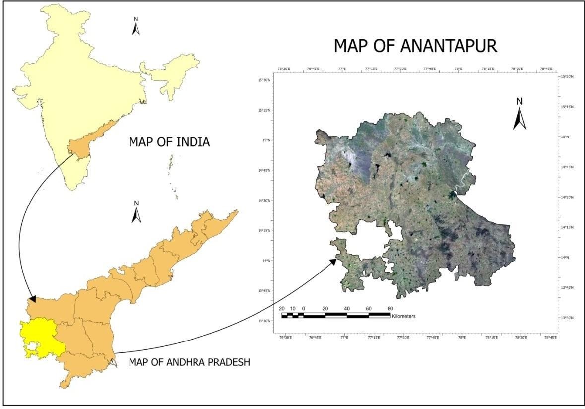
3.1 Fig. Map of study Area

 

C. Terrain

The district of Anantapur has a fair elevation, which gives the district a good climate all year long. It gradually descends from the south to the north, heading for the Pennar Valley in the Peddavadugur, Peddapappur, and Tadipatri areas. The Hindupur, Parigi, Lepakshi, Chilamathur, Agali, Rolla, and Madakasira areas in the south gradually ascend to join the Karnataka Plateau, which has an average elevation of roughly 2000 feet above mean sea level. Anantapur has a height of approximately 1100 feet, and Tadipatri has the lowest elevation of 900 feet.

Due to the peninsula's location, agricultural conditions there are frequently unstable. This area is also avoided by the monsoon because of its terrible location. It is separated from the East coast by the high Western Ghats, the South Atlantic Ocean, and the North East Monsoon, so it does not benefit entirely from such events.

 

D. Soil and Geological characteristics

The topography of the study region is undulating. The soil, composed of clay minerals, goes down 10 metres below the land's surface. The Anantapur District's geological formations can be roughly divided into two different and well-delineated groups: an older group of metamorphic rocks from the Archaean age and a younger group of sedimentary rocks from the Proterozoic period (GSI, 2001). The latter include the Tadipatri, Putlur, eastern Gooty, and Narpala regions. The remaining areas are covered in Archaean rocks such as schists, gneisses, Migmatites, newer granites, pegmatites, quartz veins, and fundamental dykes. The Archaean rocks have undergone many tectonic disturbances, which have caused metamorphism and recrystallization in the rocks.

 

E. Drainage

The Pennar River is the most significant of the rivers flowing through the area. It originated in the Nandi Hills in the Indian state of Karnataka. It travels through the Parigi, Roddam, Ramagiri, Kambadur, Kalyandurg, Beluguppa, Uravakonda, Vajrakarur, Pamidi, Peddavadugur, Peddapappur, and Tadipatri areas before entering the Cuddapah District. It first enters the Anantapur district from the far southern part of the Hindupur area. The Karnataka-born Jayamangala River enters the district through the Parigi area and merges with the Pennar River in Sangameswarampalli of the Parigi area. The Chitravathi, which also has its source in Karnataka, is a significant river in the area. This river travels north over the stony, mountainous highland before entering the Pennar River at Gandikota in the Cuddapah District. It enters the district close to Kodikonda hamlet of Chilamathur Mandal. Through the Gummagatta, Brahmasamudram, Beluguppa, Kanekal, and D. Hirehal Mandals and into the Bellary District of Karnataka State, the Vedavathi River runs. On this river, the Bhairavanithippa project has been built. In addition to these streams, others in the district include Kushavathi in Chilamathur Mandal, Swarnamukhi in Agali Mandal, Maddiler in Nallamada, Kadiri, and Mudigubba Mandals, Pandameru in Kanaganipalli, Raptadu Anantapur B.K.Samudram, and Singanamala Mandals, and Papagni in Tanakal Mandal.

 

F. Climate

Due to its distance from the East Coast and the Western Ghats mountain range, which blocks the South West Monsoon from reaching these dry soils, it does not fully benefit from the North East Monsoons. As a result, it can be seen that the area frequently experiences droughts and a lack of monsoon rains. The district receives the least amount of rainfall compared to Rayalaseema and other areas of Andhra Pradesh, with an average rainfall of 553.0 MMS. The South West Monsoon season typically receives 338.0 mm of rain, i.e., 61.2% of total precipitation. Only 156.0 mm of the year's total rainfall, or 28.3%, comes from the North East monsoon period (October to December). The remaining months are nearly dry. The average daily maximum temperature in March, April, and May is warm, ranging from 29.1 C to 40.3 C. Due to their high elevation, the Mandals of Hindupur, Parigi, Lepakshi, Chilamathur, Agali, Rolla, and Madakasira experience colder temperatures during the cooler months of November, December, and January, when the temperature drops to about 15.7 C.

 

G. Population

According to the census 2011, the District has a population of 4081148. Compared to the state's 308, the District has a lower population density of 213 people per square kilometre. According to the 2011 Census, 72% and 28% of the District's population was rural, compared to 75% and 25% in the 2001 Census. In the 2011 Census, there were 977 more females than males. According to the 2011 census, 49.89% of workers in the District and 25% work in the agricultural industry.

There are 929 inhabited villages out of 964 total revenue villages.

 

H. Vegetation

1) Plantation of agriculture

These regions have been planted with agricultural tree crops using agricultural management methods. These also include land use systems and practices where the cultivation of herbs, shrubs, and vegetable crops is purposefully integrated with crops, primarily in irrigated conditions, for ecological and economic reasons. These include, for instance, permanent commercial crops like coffee, mulberry, tea, and rubber. Which are typically grown in hilly regions and are closely associated with forest cover; plantations of berry shrubs, such as raspberry, gooseberry, and other types of berry crops; the aerial extent of this category in the Anantapuramu District is 76.24 square kilometres or 0.40% of the district's overall land area.

 

2) Forest

The total aerial extent of this category in the Anantapuramu District is 1802.42 sq km or 9.42% of the District's general geographic area. There are not many forests in the District. In the Anantapur District, the word "forest" does not connote a dense tree population or thick vegetation of varied pastures. The District's woodlands are few and thin.

 

I. Objectives

The study aims at following major objectives

1. Identifying how different natural factors affecting the agriculture.
2. Assessing the suitability criteria using AHP.
3. Creating suitability maps to analyze decision support systems.
4. To help in enhancement of rural economy, by the agricultural site suitability study.

 

IV. DATABASE AND METHODOLOGY

A. Data source

The following maps for the best allocation of suitable agricultural sites were generated using the Arc Map 10.8 version, ArcGIS Pro and QGIS software:

Table 4.1: Datasets utilized for different parameters

Serial No.	Parameters	Database	Data Type
1	Normalize Difference Vegetation Index	Landsat8	Spectral
2	Normalize Difference Moisture Index	Landsat8	Spectral
3	Elevation	SRTM	DEM
4	Slope	SRTM	Generating DEM data
5	Aspect	SRTM	Generating DEM data
6	Rainfall	CHRS	Raster
7	LULC	Landsat8	LULC
8	Soil Data	ISRIC	Raster
9	Distance from rivers	Open street maps	Raster
10	Distance from Roads	Open street maps	raster
11	LST	MODIS	RASTER

 

The datasets that have been utilized for the study after consideration of the different parameters are described below

1) Landsat8

The landsat8 data has been used for different parameters. Landsat-8 was launched in February 2013. (LDCM). This cooperative effort, run by the United States Geological Survey (USGS), aims to gather and store thermal and multispectral image data while maintaining consistency with earlier Landsat mission data. A Thermal Infrared Sensor instrument (TIRS) and Operational Land Imager (OLI) on Landsat-8 replace the Enhanced Thematic Mapper Plus (ETM+) sensor on the previous satellite (Landsat-7). The multispectral, moderate-resolution OLI instrument was created by Ball Aerospace Technology Corporation (BATC). There are nine spectral bands in OLI, including five in the visible and near-infrared spectrum (NVIR), three in the short-wave infrared spectrum (SWIR), and one panchromatic image (PAN) band for picture sharpening.

These bands cover a spectral range from 433 to 2300 nm.

 

2) MYD11A1.061 Aqua Land Surface Temperature and Emissivity Daily Global 1km

Dataset has been used to obtain the land surface temperature information for the study region. It is a level 3 product of the MODIS LST, having a spatial resolution of approximately 1 km. It is derived from the MYD11_L2 swath product. As the latitude increases and goes above 300, the sensor may record multiple observations in some pixels. The problem is corrected by determining the value of a single pixel by averaging the multiple observations. The sensor is provided with bands for recording daytime and nigh time surface temperature, and bands 31 and 32 of MODIS act as quality indicators along with six observation layers.

 

3) Openstreet map

Steve Coast created the OpenStreetMap (OSM) in 2004 to construct a geographic database that can be edited and used by users around the globe free of cost. The concept of OSM is based on crowd sourcing in which the registered users can add data they have collected using different methods to the OSM database. Such a facility has led to the creation of a robust database that people can access for their projects, the development of paper and electronic maps, geocoding addresses and other places.

Geofabrik is a company that provides software development services. It involves extracting the information from OSM and converting it to shapefile format (.shp) for convenient usage of the available datasets. For the present study, layers of roads and settlement areas were downloaded from the website of Geofabrik as line and polygon features, respectively.

 

4) Flow Diagram

The current study used multi-criterion site suitability modeling to determine appropriate and viable agricultural development places based on a set of limitations and criteria. Ten different limitations and criteria were chosen based on their significance and value in agriculture. The maximum limitation technique, which incorporates soil PH, elevation, slope, Rainfall, Land surface temperature, distance from rivers distance from roads, NDVI and NDMI was used to identify several parameters influencing agricultural product yield. Furthermore, weights for each specified criterion were computed using the analytical hierarchy approach, and the suitability map was created using the weighted overlay method. The methodological flow diagram of the present study is shown below (Pramanik, 2016).

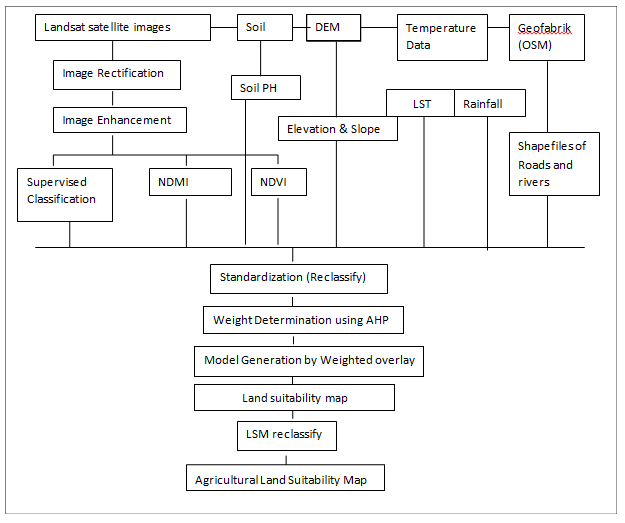
Figure4.1: Flowchart of the methodology followed for the generation of final site-suitability map

 

B. Methodology

In the study to map suitability zones in Anantapur of Andhra Pradesh, the majority of the datasets associated with the different parameters have been retrieved and computed using the USGS portal, which was then analyzed further in the ArcGIS software. Google earth engine has been used, which is a cloud-based platform which is used by scientists and other organizations around the globe for performing geospatial analysis. Soil data has been collected from World soil information. Distance from roads and settlement layers have been downloaded from the Geofabrik website in vector format. Details of each layer procured for the study are given below:

1) NDVI_max: The Normalized Difference Vegetation Index (NDVI) acts as an indicator to determine the photosynthetic activity of vegetation of a region. In short, it assesses the overall health of vegetation. The NDVI is calculated by taking the red band (red) and near-infrared band (NIR) into consideration since the chlorophyll pigment of healthy vegetation usually absorbs most of the red light and reflects more near-infrared light. Hence, the index is calculated by comparing the amount of red light absorbed and near-infrared light reflected. The formula is:

NDVI = (NIR-Red) / (NIR+Red).

NDVI calculations for a given pixel always in a number that ranges from -1 to +1. Negative values indicate water surfaces, rocks, snow etc. A value between 0.1-0.2 corresponds to bare soil, 0.2-0.5 indicates sparse vegetation and healthy vegetation is indicated by values above 0.5. The table depicts the NDVI value range along with their description.

 

Table 4.2: NDVI value range and their implications

NDVI Vaule Range	Vegetation Health
-1 to 0.1	Water bodies
1 to 0.2	Bare surfaces
0.2 to 0.5	Moderate
>0.5	Healthy

 

The NDVI_max can be defined as the best health status that can be achieved by vegetation during a single growing season. For the study, NDVI_max has been generated using the ArcGIS software. For the analysis, the data range has been taken for 2021.

 

2) NDMI (moisture): The layer has been generated using ArcGIS Software. Normalized Moisture Index is used to determine the moisture content in the vegetation. The SWIR band is capable of detecting the moisture level in the mesophyll tissue, whereas the NIR band can determine the dry matter content in the leaves. The index is therefore computed by utilizing the reflectance of near-infrared (NIR) and short-wave infrared (SWIR) and is given by the formula:

NDMI = (NIR – SWIR) / (NIR + SWIR)

Similar to NDVI, this index also generates values in the range of +1 to -1. The negative values indicate low moisture content or water-stressed vegetation, whereas values close to 1 represent water surfaces. Vegetation having low moisture content will be more susceptible to ignition due to drier conditions. For the NDMI analysis, the data range of 2021 has been taken to visualize the status of moisture concentration in vegetation for the time period.

 

3) Elevation

The DEM proved helpful for this research in identifying different landforms and describing the terrain. Although extensive mapping information was not ideal due to the data being expressed on a 36x36m grid, it is believed to be a crucial first step in guiding investigations at other farm locations.

 

4) Slope

The slope and aspect map has been derived from the DEM data analysis.

The slope layer has been generated in the ArcGIS from the elevation map using the ‘slope’ tool under the ‘spatial analyst’ tool. It is another parameter that significantly contributes to determining the site suitability of agricultural land. For determining a proper area for farmlands slope parameter is required. The slope values in the study region vary from 00 to more than 800.

 

5) Land Use /Land Cover

To make land use classification easier to understand, false-colour composite bands have been used in several satellite images. False-colour composite bands (4, 3, 2) are used in some satellite images to contrast the various land cover classifications. Six categories of land cover and land use were utilized to classify the Anantapur LULC: water, vegetation, scrub, built-up, deciduous forest, and barren land. Using supervised classification, ArcGIS software has been used to categorize land use and land cover (maximum likelihood approach). A spectral signature defines the training sets for the supervised classification, which are relevant to the entire image. The Maximum Likelihood Algorithm is used because it computes the statistics, which are generally distributed for each class in each band, and computes the likelihood for a pixel to belong to a specific class. The class with the highest probability is given to each pixel. The default mode of this algorithm is always used for supervised classification.

 

6) Land Surface Temperature

The map for land surface temperature was generated by taking the suitable land for agriculture of Anantapur in the value range. Higher values represent regions having high temperatures indicating more heat from the sun and dry environment, which increases the probability of drought occurrence, whereas lower values depict regions such as water bodies. For the study area, the lowest temperature recorded was 300k, and the highest temperature was 316K.

 

7) Rainfall

The Centre for Hydrometeorology and Remote Sensing (https://chrsdata.eng.uci.edu/) provided rainfall data for the research sites. There has been the use of PERSIAN-CCS Data. The Centre for Hydrometeorology and Remote Sensing (CHRS) at the University of California, Irvine, created the PERSIANN-Cloud Classification System (PERSIANN-CCS). This real-time, high- resolution satellite precipitation product covers the whole world (UCI). The PERSIANN-CCS method divides cloud-patch characteristics into categories based on satellite data derived from cloud height, areal expanse, and textural diversity. The core of PERSIANNCCS is the variable threshold cloud segmentation method.

 

8) Soil

Data on soil was gathered for this study from the ISRIC Portal. Various levels are used to collect soil data, including point, map unit, spatial, and interpretive data. Point data, which is site- specific and represents a Pedon profile, ought to demonstrate the best features of a specific soil. The information in map units talks about the terrain, climate, flora, and geology, as well as the locations of different soil types in each area and how they are interrelated, as well as how they differ in terms of colour and texture. The georeferenced ortho quadrangle base map contains soil delineations and distinguishing characteristics as spatial data.

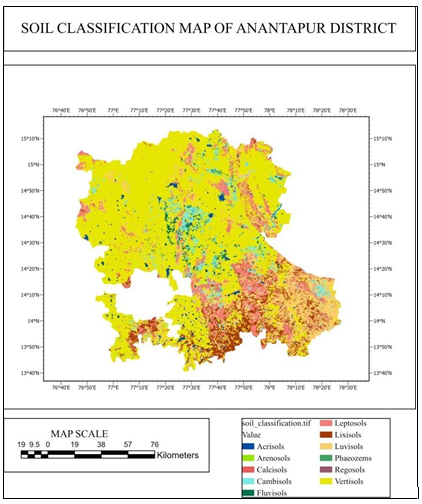
Fig4.2. Showing the soil classification of the district

 

9) Distance from roads

The shapefiles of the road layer were downloaded from the Geofabrik website, which was then visualized in the GIS environment, i.e. in ArcGIS software, after which the layer was extracted for the study area. The Euclidean distance tool was then run on the layer, generating the Euclidean distance surface rasters for roads. The tool can measure the distance between each pixel from its nearest source, which can give us an idea about the areas located near roads.

 

10) Distance from rivers

The shapefiles of the settlement area were downloaded from the Geofabrik website, which was then visualized in the GIS environment, after which the layer was extracted for the study area. The Euclidean distance tool was then run on the layer, generating the Euclidean distance surface rasters for river areas. The distance of each pixel from its nearer source can be measured with the tool, which can give us an idea about the areas located close to river areas.

GIS is a computer-based system capable of handling practically any kind of data regarding attributes that may be linked to a specific geographic area. The capacity of GIS to meaningfully and effectively spatially interrelate various types of information originating from a variety of sources is one of its most significant advantages.

The Ten maps generated were reclassified by their values in ArcGIS to obtain a different number of classes for each parameter.

The present study attempts to assess the agricultural suitability zones in Anantapur, which is associated with ten parameters considered that have influence over natural factors’ behavior. The Analytic Hierarchy Process or AHP has been used to carry out the analysis. The Analytic Hierarchy Process (AHP) was developed by Thomas L. Saaty in the 1970s, and it is a widely used method which combines mathematics and psychology. The method has been extensively utilized for multi-criteria decision-making (MCDM), which can be defined as taking a decision about solving a particular objective when there is the involvement of multiple criteria.

The process is composed of three different steps described as follows:

Step 1) Development of a hierarchical structure by keeping the primary objective at the first level, criteria at the second level and alternatives at the third level

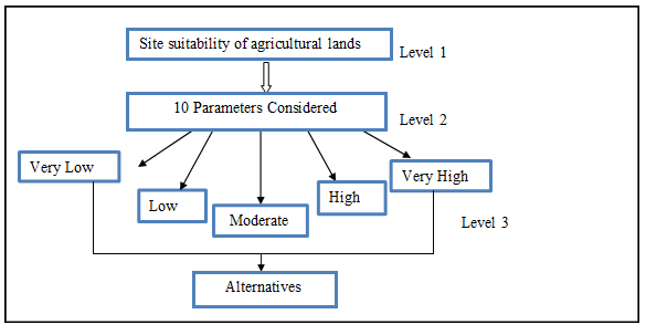
The primary objective is to identify the site suitability of agricultural lands in different parts of the state, which is placed at level 1. The ten parameters or criteria based on which the decision will be made placed at level 2. Level 3 represents five alternatives, viz. very low, low, moderate, high and very high, associated with each parameter.

 

Step 2) Determination of the relative importance of the different parameters by taking into account the primary objective

For the second step, a pairwise comparison matrix was constructed to assign relative importance to each parameter by considering the goal of identifying site-suitable zones. Two parameters were compared each time, and a value was assigned based on the importance of one parameter in land evaluation mapping concerning the other factor. The matrix was created by using the scale of relative importance. The table depicts the scale containing their values along with an explanation and description. The values have been assigned after a thorough literature review and in consultation with the experts.

 

Table4.3: Scale of relative importance for AHP

Intensity of Importance	Definition	Explanation
1	Equal importance	Two elements contribute equally to the objective
3	Moderate importance	Experience and judgment slightly favor one element over another
5	Strong importance	Experience and judgment strongly favor one element over another
7	Very strong importance	One element is favored very strongly over another, it dominance is demonstrated in practice
9	Extreme importance	The evidence favoring one element over another is of the highest possible order of affirmation
2,4,6,8 can be used to express intermediate values 1/3,1/5,1/7,1/9 are used to express reverse comparison

 

Table 4.4: Pair wise comparison matrix

		Pair-wise comparison matrix
Sl.no .	Parameters	NDVI_ma x	NDMI	Elevatio n	Slope	soil	LuLc	Distance from river	Distance from road	Land Surface Temperature	Rainfall
1	NDVI_max	1.00	0.50	0.33	0.33	0.50	0.33	0.33	0.25	0.20	0.13
2	NDMI	2.00	1.00	0.50	0.50	0.50	0.50	0.25	0.33	0.17	0.13
3	Elevation	3.00	2.00	1.00	0.33	0.50	0.33	0.33	0.33	0.14	0.13
4	Slope	3.00	2.00	3.00	1.00	0.50	0.50	0.50	0.20	0.20	0.11
5	Soil Ph	2.00	2.00	2.00	2.00	1.00	0.33	0.33	0.33	0.17	0.11
6	LULC	3.00	2.00	3.00	2.00	3.00	1.00	0.33	0.33	0.25	0.14
7	Distance from river	3.00	4.00	3.00	4.00	3.00	3.00	1.00	1.00	0.20	0.13
8	Distance from road	4.00	3.00	3.00	5.00	3.00	3.00	1.00	1.00	0.17	0.13
9	Land Surface Temperature	5.00	6.00	7.00	5.00	6.00	4.00	5.00	6.00	1.00	0.20
10	Rainfall	8.00	8.00	8.00	9.00	9.00	7.00	8.00	8.00	5.00	1.00
	SUM	34.00	30.50	30.83	29.17	27.00	20.00	17.07	17.77	7.50	2.21

 

 

In table 4.4, two parameters were taken into consideration at a time for the assignment of a value in each call. For instance, in the first cell, both the parameters are identical, due to which value one has been assigned to the cell. In the next row, two parameters are the vegetation index and the moisture index. The value has been assigned based on whether the moisture parameter significantly influences site suitability mapping over the vegetation index. Value 2 assigned to the cell indicates that even though both parameters contribute almost equally to site suitability mapping, the moisture parameter's importance is slightly more than the NDVI_max.

Similarly, the other cells in the lower half of the diagonal were filled by pairwise comparison. Based on the filled values, the cells in the upper portion of the diagonal were filled by reversing the corresponding values. For example, if NDMI is two times more important than NDVI in suitability mapping, NDVI will be ½ or 0.5 times more critical than NDMI. After this, each column was summarized, and the element of each column was divided by the sum of the values in the corresponding column to generate the normalized pairwise comparison matrix. The criteria weights were then calculated for each parameter to understand their relative importance in Land evaluation mapping by adding the elements of each row and dividing them by the number of criteria (10).

 

Table 4.5: Criteria weights derived for each parameter after completion of Step 2

Parameters                                                                                            Criteria Weights
NDVI_max	0.02 0.03 0.03 0.04 0.04 0.06 0.09 0.09   0.20   0.38
NDMI
Elevation
Slope
Soil
Land Use/Landcover
Distance from river
Distance from road
Land Surface Temperature
Rainfall

 

Step 3) Calculation of consistency to check whether the criteria weights obtained are correct or not. The matrix that was not normalized was taken, and elements of each column were multiplied by respective criteria weights, and the values in each row were added to obtain the weighted sum value as depicted in table 6.4. The ratio of the weighted sum value to the criteria weight for each row was calculated

 

		Calculation of consistency of the pair wise comparison matrix
Sl.no.	Parameters	NDVI_max	NDMI	Elevation	Slope	soil	LULC	Distance from river	Distance from road	Land Surface Temperature	Rainfall	Weighted sum value	criteria weights	ratio
1	NDVI_max	1.00	0.50	0.33	0.33	0.50	0.33	0.33	0.25	0.20	0.13	0.25	0.02	11.13
2	NDMI	2.00	1.00	0.50	0.50	0.50	0.50	0.25	0.33	0.17	0.13	0.30	0.03	10.62
3	Elevation	3.00	2.00	1.00	0.33	0.50	0.33	0.33	0.33	0.14	0.13	0.35	0.03	10.12
4	Slope	3.00	2.00	3.00	1.00	0.50	0.50	0.50	0.20	0.20	0.11	0.45	0.04	10.32
5	Soil	2.00	2.00	2.00	2.00	1.00	0.33	0.33	0.33	0.17	0.11	0.46	0.04	10.80
6	LULC	3.00	2.00	3.00	2.00	3.00	1.00	0.33	0.33	0.25	0.14	0.67	0.06	10.82
7	Distance from river	3.00	4.00	3.00	4.00	3.00	3.00	1.00	1.00	0.20	0.13	1.04	0.09	11.39
8	Distance from road	4.00	3.00	3.00	5.00	3.00	3.00	1.00	1.00	0.17	0.13	1.07	0.09	11.40
9	Land Surface Temperature	5.00	6.00	7.00	5.00	6.00	4.00	5.00	6.00	1.00	0.20	2.54	0.20	12.55
10	Rainfall	8.00	8.00	8.00	9.00	9.00	7.00	8.00	8.00	5.00	1.00	4.76	0.38	12.53
SUM														111.68
Table 4.6: Calculation of consistency of the pair wise comparison matrix

 

                                                                

Calculation of the consistency ratio (CR):

The consistency ratio (CR) is calculated through several steps. The matrix will be accepted if the value of CR remains below the value of 0.10, or the matrix will be rejected. We would need to find alternative ways to compute the values. The steps involved in the calculation of CR are as follows: The Lambda_max (Λmax) was calculated by averaging the ratio column and is given by:

 

Λmax = 111.68/10 = 11.168

 

After this, the consistency index (C.I.) was computed which is given by the formula:

C.I.= (Λmax-n) / (n-1)

 

Here, n is the number of elements compared i.e., 10 Therefore, the consistency index is calculated as:

C.I. = (11.168-10) / (10-1) = 0.129

The C.R. was calculated by taking the consistency index (C.I.) and dividing it by a random index (R.I.). The random index is the consistency index of a randomly generated pairwise matrix.

Table 6.5 represents the random index (R.I.) value corresponding to the number of criteria involved (n) obtained from the internet.

 

Table 4.7: Random Index table corresponding to different criteria

n	1	2	3	4	5	6	7	8	9	10	11
RI	0.00	0.00	0.58	0.90	1.12	1.24	1.32	1.41	1.45	1.49	1.51

 

Since, 10 criteria are involved in the study i.e., n = 10, the value 1.49 would be computed as random index in the calculation of consistency ratio.

The consistency ratio was calculated as:

CR = CI / RI = 0.129/1.49 = 0.087

 

The CR value indicates that the inconsistency proportion is less than 0.10. Thus, it can be assumed that the matrix is reasonably consistent. The criteria weights obtained are valid and can be further used for decision-making.

Each parameter was categorized into several classes. Each class was given a rank based on their land evaluation degree and criteria weights derived from AHP, as depicted in table 4.6. The rankings were based on five different levels of site suitability, as represented in table 4.8.

Table 4.8: Different levels of suitability of land

Suitability Level	Rating
Very Low	1
Low	2
Moderate	3
High	4
Very High	5

 

Table 4.9: Ranking of classes of different parameters based on site –suitability of land

SL No.	Variables	Weight Factor(f rom AHP)	Classes	Rating	Site- suitability
1	Elevation(m)	0.03	0 - 300	5	Very High
			300.001 - 420	4	High
			420.001 - 510	3	Moderate
			510.001 - 600	2	Low
			600.001 - 960	1	Very Low
2	Slope(degree)	0.04	0-2.24	5	Very High
			2.25-6.72	4	High
			6.73-13.90	3	Moderate
			13.91-22.86	2	Low
			22.87-57	1	Very Low
3	NDVI_max	0.02	-1-0.1	1	Very Low
			0.1-0.2	1	Very Low
			0.2-0.5	4	High
			>0.5	5	Very High
4	LULC	0.06	Built-up area	2	Low
			Agricultural Land	5	Very High
			Scrub Land	3	Moderate
			Deciduous Forest	4	High
			Barren Land	2	Low
			Water Bodies	1	Very Low
5	NDMI(-1+1)	0.03	0-0.48	1	Very Low
			0.48-0.63	2	Low
			0.63-0.73	3	Moderate
			>0.73	4	High
6	Soil PH	0.04	<=6	1	Very Low
			<=6.5	1	Very Low
			<=7	2	Low
			<=7.5	2	Low
			<=8	5	Very High
7.	Distance from roads	0.09	0 - 1,918.52	1	Very Low
			1,918.52 - 3,837.05	2	Low
			3,837.05 - 5,755.58	3	Moderate
			5,755.58 - 7,674.11	5	Very High
8	Distance from Rivers	0.09	0 - 0.06278	5	Very High
			0.06278 - 0.12556	4	High
			0.12556 - 0.18835	3	Moderate
			0.18835 - 0.25113	1	Very Low
9	Land Surface Temperature	0.20	300.1139 - 304.8241	5	Very High
			304.8241 - 306.9882	4	High
			306.9882 - 309.5979	3	Moderate
			309.5979 - 316.3450	1	Very Low
10	Rainfall(mm)	0.38	635.701 - 677.727	1	Very Low
			677.728 - 705.019	2	Low
			705.02 - 747.046	2	Low
			747.047 - 811.765	3	Moderate
			811.766 - 911.427	4	High
			911.428 - 1,064.899	5	Very High

 

 

V. RESULTS AND DISCUSSIONS

A. Generation of layers of parameters involved in site suitability mapping

1) NDVI_max:

Assessing vegetation health is crucial in determining areas most suitable for agriculture. The classification of NDVI values into several value ranges helps in the identification of what each of the value ranges represents. Since the map has been generated by filtering the date range for the year 2021 in Anantapur, in figure 5.1, we can observe that a significant part of the vegetation has good health due to the presence of some forest covers in that area. The total area is covered with moderate healthy vegetation, the agricultural lands depicted by light green colour. The built-up areas/ barren land with no vegetation is depicted in red. The NDVI_max value, the best possible health the vegetation can achieve during the summer and autumn seasons has been used in the study to understand the influence of the climate.

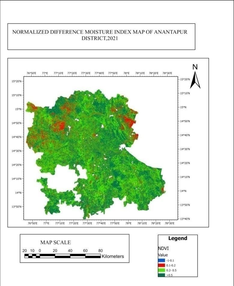
FIG.5.1 NDVI MAP OF ANANTAPUR DISTRICT

 

2) NDMI (Moisture)

The moisture index helps determine moisture content in the study area. It is specifically helpful in assessing the moisture present in vegetation. The presence of moisture is critical in influencing crop conditions in the area. Dry vegetation will be unhealthy compared to vegetation with a high moisture concentration. In figure 5.2, a low value of NDMI is associated with low moisture content and water-stressed areas most likely to be affected by droughts.

On the other hand, a high value of NDMI is related to higher moisture concentration which puts those areas at very low or no risk of droughts. The negative and shallow values of NDMI indicate areas vulnerable to forest fire risk since the absence of moisture can provide the risk of droughts. Very high NDMI values, as depicted by darker shades of blue, signify the presence of water bodies.

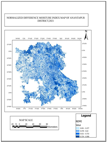
FIG 5.2. NDMI MAP OF ANANTAPUR DISTRICT

 

3) Elevation

The digital elevation model (DEM) generated for the study area contains the elevation data. The elevation is another factor that can highly influence site suitability for agricultural land. The increase in temperature is inversely proportional to the increasing elevation, which can significantly reduce the chances of the incidence of a low suitable agricultural land. Altitude also plays an essential role in influencing the vegetation structure and type of climate. In figure 5.3, the elevation values have been classified into five classes in ascending order which can help to visualize how the elevation is changing throughout the state. The map indicates that areas having low altitudes are situated in the Northern part of the state. In contrast, the area has a high elevation in the Southern part.

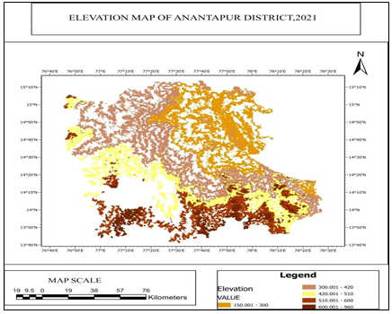
FIG 5.3 ELEVATION MAP OF ANANTAPUR DISTRICT

 

4) Slope

The slope of an area is associated with its steepness. A high value of slope implies higher steepness of the ground surface. The slope is determined by calculating the tangent of a surface. It is measured by dividing the vertical change in elevation (perpendicular) by the horizontal distance (base). Greater steepness lowers the suitability of agricultural lands. Figure 5.4 shows that yellow portions indicate areas with significantly lower slope values. The slope value increases considerably with increasing altitude and is very high (as represented by red) in the mountainous southern portion of the state.

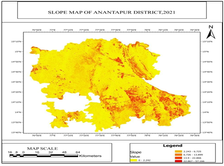
FIG5.4. SLOPE MAP OF ANANTAPUR DISTRICT

 

5) Land Cover/Land Use

Understanding the landscape of a region is very important in evaluating agricultural lands. Land cover refers to a region's natural cover, including forests, river streams, etc. On the other hand, land use is defined as the land area used by humans for different purposes such as agriculture, recreational activities, etc.

Information on land cover enables sustainable land management by preventing cultivation or developments in areas already used for a particular purpose or are important biologically and ecologically. Many aerial photos feature land-use classifications made using false-colour composite bands. False-colour composite bands are used in several aerial photos, and false- colour composite bands are used to compare different land cover categories. The six-land use/land cover classes used for LULC categorization are Water bodies, Deciduous Forests, Bare Lands, Agriculture, Scrub, Built-up Areas, and Others. The arc map software used supervised classification (a maximum likelihood approach) to categorize land use and land cover.

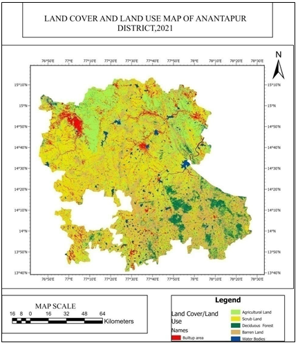
FIG 5.5 LULC MAP OF ANANTAPUR DISTRICT

 

6) Soil Ph

The pH of the soil will have an impact on how the nutrients interact with one another as well as how readily available they are to plants. It influences plant growth and the soil's physical, chemical, and biological qualities and processes. Most crops' nutrition, growth, and yields decline in environments with low pH and climb as pH approaches its ideal level. Because most plant nutrients are readily available in this pH range, a pH range of 6 to 7 is typically the most favorable for plant growth. Some plants, however, require soil pH levels above or below these limits. Calcium, magnesium, and phosphorus are typically less available in soils with a pH below

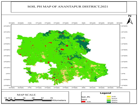
FIG5.6 SOIL PH MAP OF ANANTAPUR DISTRICT

 

7) Rainfall
A direct link exists between agriculture and rainfall. Therefore, changes in rainfall patterns have a direct impact on crop patterns all over the world. The district receives 520 mm of rainfall on average each year, with 0 mm in February and March and 129 mm in September. The wettest months of the year are September and October. The average seasonal rainfall ranges from 1 mm in winter (Jan-Feb) to 311 mm in the south-west monsoon (June-September), 146 mm in the northeast monsoon (Oct.-Dec.), and 72 mm in summer (March-May). (CGWB, 2013). This diagram shows that most rainfall occurs in the southern part of the district, which has come to the lowest number in the extreme northern part of the district.

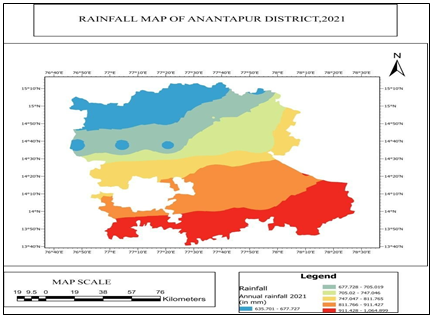
FIG5.7. RAINFALL MAP OF ANANTAPUR DISTRICT

 

8) Distance from Rivers

Rivers play a significant role in agriculture Land. Since rivers transport a variety of nutrient-rich materials and deposit them nearby, making the area around them more fertile and valuable for agriculture, rivers are another form of crop irrigation. So, from the point of crop fertility, croplands should be closer to rivers. Here, the range of 0.001 - 0.024 in light blue depicts the closest to the river beds, whereas values in deep blue (0.135 - 0.251) imply the farthest.

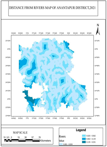
FIG5.8 DISTANCE FROM RIVERS MAP OF ANANTAPUR DISTRICT

 

9) Distance from roads

The distance from roads to agricultural areas is an essential determinant of fire risk since the availability of roads is associated with human interference. Road networks in agricultural lands can increase the accessibility by humans, which increases the probability of unhealthy and less land. Additionally, those highways are crucial for the district's communication and agricultural product transportation. However, it is possible that the placement of agricultural fields along the main metal roadways will not support the improvement of crop quality. In order to prevent the site from directly across Anantapur main routes, another Euclidian Distance for roads was created.

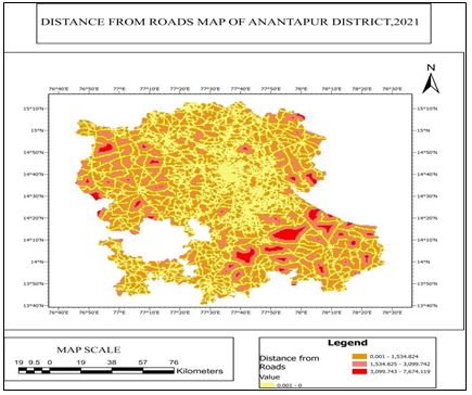
FIG5.9 DISTANCE FROM ROADS MAP OF ANANTAPUR DISTRICT

 

10) Land Surface Temperature

Out of all the parameters considered, the temperature is one of the crucial factors that primarily influence Crop behavior. High temperature implies more sunlight exposure and low precipitation, which can ultimately lead to a dry environment. In high-temperature areas, the moisture content in the vegetation cover is also low, which can act as an ideal situation for drought. Figure 5.10 shows how the land surface temperature varies throughout the state. The Anantapur region in the south experiences shallow temperatures, and the temperature increases towards the Northern part in the low-lying areas, as represented by shades of brown and red.

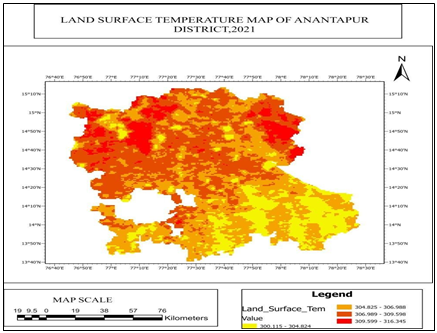
FIG5.10 LAND SURFACE TEMPERATURE MAP OF ANANTAPUR DISTRICT

 

B. Land Evaluation Of Parameter Based

1) Rainfall

This parameter is the highest influencing parameter of all. Suitable agricultural lands mainly depend on the amount of rainfall in that area. Here, it can be seen that the difference in the amount of rain is distributed all over the state. Precipitation is measured in mm. A low amount of rainfall is experienced in the Northern hilly side of the state. In comparison, it is slowly growing with the central part towards the southern area of the state. The amount of rainfall classes has been measured where low rainfall leads to a quiet, suitable area and grows towards the south from a moderate to High suitability.

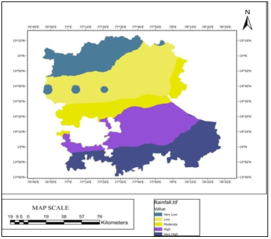
FIG5.11 RAINFALL RISK MAP OF ANANTAPUR DISTRICT

 

2) Land Surface Temperature

The land surface temperature (measured in Kelvin) significantly influences the land suitability for agriculture. As mentioned in the previous discussions, a higher temperature is associated with exposure to direct solar radiation, low precipitation and drier climatic conditions. Figure 5.12 indicates that drought risks increase proportionally with temperature. Regions experiencing higher temperatures are classified as 'Low suitability' zones. In contrast, with the drop in temperature towards the Southern part of the state, land suitability increases considerably from 'moderate' to 'very high.

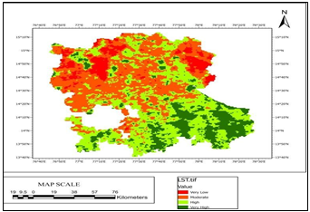
FIG5.12 LAND SURFACE TEMPERATURE RISK MAP OF ANANTAPUR DISTRICT

 

3) NDVI_max

The vegetation health during the Land evaluation is on the excellent side, i.e. mostly healthy vegetation with minimal moisture content. Hence, from February to December, a significant portion of the state has healthy foliage (as depicted in figure 5.13). The amount of unhealthy vegetation has comparatively low, mostly seen on the northern side. The water bodies, barren areas devoid of vegetation, have no input for land evaluation. Hence, they have been classified under the 'very Low' class.

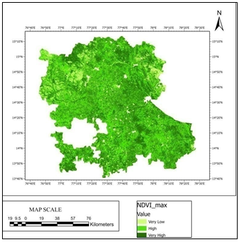
FIG5.13 NDVI RISK MAP OF ANANTAPUR DISTRICT

 

4) NDMI (moisture)

The normalized difference in moisture index determines the moisture concentration in vegetation. Figure 5.14 represents the state vulnerable to different levels of Land suitability. Regions with low values of NDMI are dry regions categorized as ‘high’ suitable areas, whereas moderate NDMI values imply sites have ‘moderate’ land suitability. On the other hand, water bodies have ‘High’ usefulness since they have high NDMI values, which is advantageous for plantation.

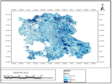
FIG5.14 NDMI RISK MAP OF ANANTAPUR DISTRICT

 

C. Model Builder

A GIS analyst and data scientist Emmanuel Jolaiya presents ModelBuilder in ArcGIS, which can be used to create models for evaluating and working with GIS data. A model is shown as a diagram, flowchart, or workflow that links a series of operations and Geoprocessing tools, utilizing the results of one function as the input to another. It allows you to construct and share your models as tools, offering advanced ways to extend GIS features.

A model builder has been used to iterate the complete model using an iterator and determine the workflow model to repeat the entire procedure. Using a raster calculator, all the input criterion layers—including elevation, slope, LULC, soil moisture, vegetation, rainfall, soil ph, river, and road—have been inserted and then classed into a single unit. Finally, the composite map was produced using the weighted overlay tool.

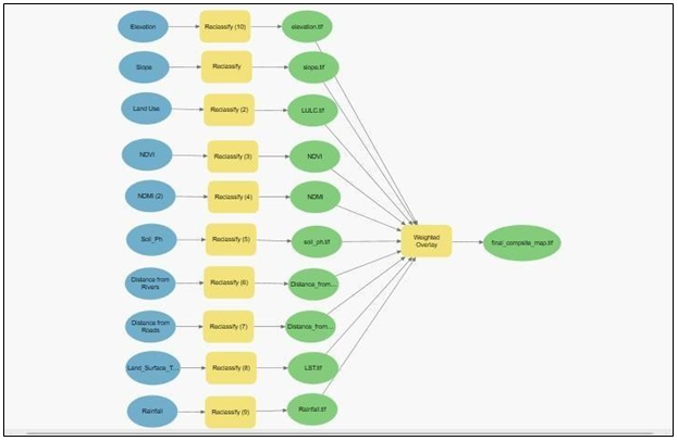
FIG5.15 MODEL BUILDER

 

1) Ranking system based on land suitability factors:

Out of the ten parameters considered, each was ranked based on their importance in influencing land evaluation, as in figure5.15. The weights were derived from AHP, indicating that the Rainfall is the highest factor of all as it is a drought-prone region and also primary need for vegetation is water. The temperature has the second highest amount of matter to determine land suitability since high temperature provides an unfavorable situation for the crops causing droughts. Land use/land cover is also critical since the type of vegetation in an area is essential to assessing land suitability. Distance from roads and rivers almost have the same degree of importance since they consider anthropogenic activities. Elevation and Slope have the same weightage to influence a land evaluation. Even though moisture and vegetation health have been given less weightage compared to other parameters, they are also crucial for evaluating land suitability. Apart from this, Soil Ph is also a critical influencing factor here.

 

TABLE5.1 ranking of the parameters based on their degree of importance to influence land suitability

Rank	Parameter	Weightage (%)
1	Rainfall	37.8
2	Land surface Temperature	20.24
3	Distance From Rivers	9.41
4	Distance From Roads	9.14
5	Land Use/Landcover	6.18
6	Soil Ph	4.32
7	Slope	4.23
8	Elevation	3.48
9	NDMI (moisture)	2.81
10	NDVI_max(vegetation)	2.2

 

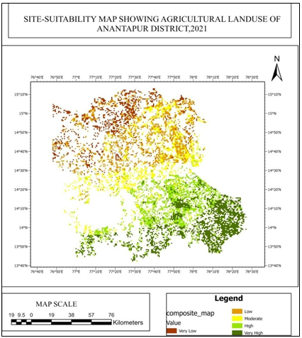
FIG5.16. SITE-SUITABILITY MAP OF AGRICULTURAL LAND OF ANANTAPUR DISTRICT

 

Figure 5.16 it represents the different suitable zones based on their different influencing parameters. The final suitability map has been prepared at a 1 km spatial resolution. In table 5.1, thearea falling under each suitable zone has been calculated in ArcGIS by the formula:

 

Area (sq.km) = Spatial resolution x Total counts = 1 x Total counts

 

Therefore, Area (sq.km) = Total counts

The table shows that the highest percentage of the area falls under the ‘high’ risk zone followed by ‘very high’ ‘, low’, and ‘High’ suitable zones, respectively.

Table 5.2: Distribution of area under each risk zone

Suitability	Percentage(%)
Very Low	11.88
Low	23.27
Moderate	17.20
High	22.52
Very High	25.13

 

D. Discussions

A GIS method called overlay mixes various data sets to find connections between them. An overlay has created a composite map by fusing the geometry and characteristics of the input data sets. Arc GIS software has utilized tools like the model builder, overlay analysis, and analytical hierarchy process to overlay both vector and raster data requirements.

According to the map, 25.13% (1785.82sq km) of the research area is highly suitable, 22.52% (1599.52sq km) is quite eligible, 17.20% (1221.11 sq km) is moderately relevant, and 23.27% which is (1652.6 sq km) is marginally suitable. In comparison, 11.88% (843.7 sq km) of the land is unfit for agricultural production in the Anantapur District.64.85 per cent of the district's total area is available for agricultural land, which falls mainly in the southern part of the district.

Conclusion

Determination of site-suitability areas was done by factoring natural and anthropogenic parameters, namely vegetation health, moisture index, forest density, land surface temperature, land use/land cover, elevation, slope, aspect, and distance from roads and settlements. Analytic Hierarchy Process (AHP) was adopted to calculate the subjective weights of each parameter to understand their degree of influence on fire occurrence. At first, a hierarchy was formed by keeping the primary objective at first criteria at the second and alternatives at the third level respectively. Next, a pairwise comparison was constructed to compare two parameters simultaneously to obtain criteria weights for each layer. Lastly, the consistency ratio was calculated to evaluate the validity of the matrix. Through AHP, the relative weights obtained indicate that land surface temperature and Rainfall parameters hold more than 50% weight age in influencing a site-suitable event. Five suitability categories were derived from very low to very high based on each parameter\'s suitability capability. Classes of each layer were given a rank based on their suitability. The layers were then integrated with a GIS platform (ArcGIS for the present study) to generate a site-suitability map of each layer. Each coating was multiplied by its respective criteria weights derived from the AHP method. Then the ten layers were combined in ArcGIS to produce the suitability map of Anantapur. The research shows that 64.85% of the area is appropriate for agricultural use in the context of an application. Currently, some of these places are underutilized, swamped, or covered in shrubs; therefore, they must concentrate on development with the active involvement of farmers in the specific site without endangering the natural environment (Weerakoon, 2014). However, the low yield is brought on by geomorphologic issues, such as a very high elevation, a high degree of slope, the presence of exposed rocks, low soil moisture, and the limited accessibility of irrigation systems. Only a fixed percentage of the land in the study district has been designated as attainable for agricultural development due to all of these dangers. It is an under developed area and its economy is entirely agrarian and is characterized by aridity and drought risk. The greatest barrier to agriculture is a lack of irrigation infrastructure. 90% of the 27.5 lakh acres under cultivation are rainfed and frequently subject to drought. Additionally, there are essentially no industrial employment prospects and very little industrial development. The available livelihoods are, therefore, woefully inadequate for the rural population, and they are also extremely vulnerable. A study was carried out to determine agriculture suitability levels in some of the most critical nature reserves having high ecological importance. The result indicates that the area is vulnerable to drought and other parameters due to its climatic condition. Climate change and accelerated desertification highlight the fragility of rural livelihoods, particularly rainfed farmers. At present, which is of significant concern and the stakeholders, should address the issue. 1) Create and encourage adaptation tactics for farmers to handle the escalating climate change and variability. 2) Develop watersheds, protect the environment, and manage natural resources sustainably to stop desertification. The study was undertaken to assess the different land suitability for agriculture prevailing throughout the state. It is crucial to safeguard this priceless resource since soil health is essential to the continued sustainability of agriculture. Farmers are gradually moving away from rainfed agriculture practices toward poly cropping under zero-budget natural farming (ZBNF). The goal of poly cropping is to drought-proof dry land agriculture, which entirely depends on rainfall. The result would enable the agriculture officials and other concerned authorities to implement stringent actions and formulate better management plans on farming land for effective control to adopt potential impacts of climates and other parameters in the near future.

References

[1] Abdelrahman, M. A. E., Natarajan, A., & Hegde, R. (2016). Assessment of land suitability and capability by integrating remote sensing and GIS for agriculture in Chamarajanagar district, Karnataka, India. Egyptian Journal of Remote Sensing and Space Science, 19(1), 125–141. https://doi.org/10.1016/j.ejrs.2016.02.001 [2] Ahmed, G. B., Shariff, A. R. M., Balasundram, S. K., & Fikri Bin Abdullah, A. (2016). Agriculture land suitability analysis evaluation based multi criteria and GIS approach. IOP Conference Series: Earth and Environmental Science, 37(1). https://doi.org/10.1088/1755-1315/37/1/012044 [3] Akinci, H., Özalp, A. Y., & Turgut, B. (2013). Agricultural land use suitability analysis using GIS and AHP technique. Computers and Electronics in Agriculture, 97, 71–82. https://doi.org/10.1016/j.compag.2013.07.006 [4] Hossen, B., Yabar, H., & Mizunoya, T. (2021). Land Suitability Assessment for Pulse ( Green Gram ) Production through Remote Sensing , GIS and Multicriteria Analysis in the Coastal Region of Bangladesh. [5] Karimi, F., Sultana, S., Babakan, A. S., Royall, D., Karimi, F., Sultana, S., Babakan, A. S., & Royall, D. (2018). Papers in Applied Geography Land Suitability Evaluation for Organic Agriculture of Wheat Using GIS and Multicriteria Analysis Land Suitability Evaluation for Organic Agriculture of Wheat. Papers in Applied Geography, 0(0), 1–17. https://doi.org/10.1080/23754931.2018.1448715 [6] Kazemi, H., & Akinci, H. (2018). Short communication A land use suitability model for rainfed farming by Multi-criteria Decision- making Analysis ( MCDA ) and Geographic Information System ( GIS ). Ecological Engineering, 116(September 2017), 1–6. https://doi.org/10.1016/j.ecoleng.2018.02.021 [7] Mangan, P., Pandi, D., Haq, M. A., Sinha, A., Nagarajan, R., Dasani, T., Keshta, I., & Alshehri, M. (2022). Analytic Hierarchy Process Based Land Suitability for Organic Farming in the Arid Region. [8] Mishra, A. K., Deep, S., & Choudhary, A. (2015). Identification of suitable sites for organic farming using AHP & GIS. The Egyptian Journal of Remote Sensing and Space Sciences, 18(2), 181–193. https://doi.org/10.1016/j.ejrs.2015.06.005 [9] Orhan, O. (2021). Land suitability determination for citrus cultivation using a GIS-based multi-criteria analysis in Mersin, Turkey. Computers and Electronics in Agriculture, 190(April), 106433. https://doi.org/10.1016/j.compag.2021.106433 [10] Pramanik, M. K. (2016). Site suitability analysis for agricultural land use of Darjeeling district using AHP and GIS techniques. Modeling Earth Systems and Environment, 2(2), 1–22. https://doi.org/10.1007/s40808-016-0116-8 [11] Ramamurthy, V., Reddy, G. P. O., & Kumar, N. (2020). Assessment of land suitability for maize (Zea mays L) in semi-arid ecosystem of southern India using integrated AHP and GIS approach. Computers and Electronics in Agriculture, 179(May), 105806. https://doi.org/10.1016/j.compag.2020.105806 [12] Saha, S., Sarkar, D., Mondal, P., & Goswami, S. (2020). GIS and multi ? criteria decision making assessment of sites suitability for agriculture in an anabranching site of sooin river , India. Modeling Earth Systems and Environment, 0123456789. https://doi.org/10.1007/s40808-020-00936-1 [13] Sarkar, D., Saha, S., Maitra, M., & Mondal, P. (2022). Jo ur na l P re r f. Artificial Intelligence in Geosciences. https://doi.org/10.1016/j.aiig.2022.03.001 [14] Seyedmohammadi, J., Sarmadian, F., Jafarzadeh, A. A., & McDowell, R. W. (2019). Development of a model using matter element, AHP and GIS techniques to assess the suitability of land for agriculture. Geoderma, 352(May), 80–95. https://doi.org/10.1016/j.geoderma.2019.05.046 [15] Ustaoglu, E., Sisman, S., & Ayd?noglu, A. C. (2021). Determining agricultural suitable land in peri-urban geography using GIS and Multi Criteria Decision Analysis (MCDA) techniques. Ecological Modelling, 455(May), 109610. https://doi.org/10.1016/j.ecolmodel.2021.109610 [16] Weerakoon, K. (2014). Suitability Analysis for Urban Agriculture Using GIS and Multi- Criteria Evaluation. International Journal of Agricultural Science and Technology, 2(2), 69. https://doi.org/10.14355/ijast.2014.0302.03 [17] Yalew, S. G., van Griensven, A., Mul, M. L., & van der Zaag, P. (2016). Land suitability analysis for agriculture in the Abbay basin using remote sensing, GIS and AHP techniques. Modeling Earth Systems and Environment, 2(2), 1–14. https://doi.org/10.1007/s40808-016-0167-x [18] https://www.sourcetrace.com/blog/changing-rainfall-patterns-effect-agriculture/ [19] http://af-ecologycentre.org/ananthapur/challenges-in-anantapur-rural-areas/

Copyright

Copyright © 2024 Sukanya De. This is an open access article distributed under the Creative Commons Attribution License, which permits unrestricted use, distribution, and reproduction in any medium, provided the original work is properly cited.